| Site1 | |
|---|---|
| Sp. 1 | 4 |
| Sp. 2 | 300 |
| Sp. 3 | 56 |
| Sp. 4 | 23 |
Community Assembly and Species Coexistence
For over a century, field ecologists have been characterizing patterns in ecological communities and trying to draw theoretical inferences from the resulting data.
Central Questions:
Why do species occur in specific locations?
Why do some species coexist while others do not?
- Environmental filtering:
- Ecologically similar species should coexist in ecologically similar environments.
- Limiting similarity:
- Ecologically dissimilar species should coexist because too similar species competing for the same resources cannot stably coexist.
- Neutral theory:
- Dispersal and stochastic demographic processes explain species coexistence and species differences are not important.
1a) First-order properties of single communities
A vector of species abundance
Species composition
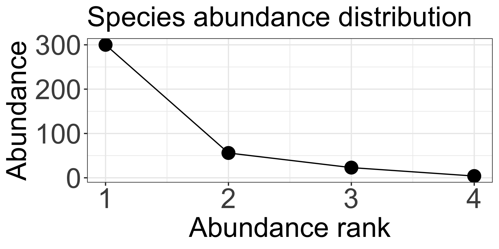
- Species richness = 4
- Simpson’s evenness = 1/ Σfreqi2 = (4/383)2 + (300/383)2 + (56/383)2 + (23/383)2
1a) First-order properties of single communities
Which community is more diverse?
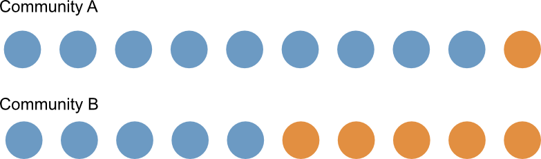
Species richness = 2
What is the chance to get the same species?
A: \(\frac{9}{10} \times \frac{8}{9} + \frac{1}{10} \times \frac{0}{9} = 0.8\)
B: \(\frac{5}{10} \times \frac{4}{9} + \frac{5}{10} \times \frac{4}{9} \simeq 0.44\)
1a) First-order properties of single communities
Which community is more diverse?
A: \(\frac{9}{10} \times \frac{8}{9} + \frac{1}{10} \times \frac{0}{9} = 0.8\)
B: \(\frac{5}{10} \times \frac{4}{9} + \frac{5}{10} \times \frac{4}{9} \simeq 0.44\)
We prefer that large values indicate more diverse communities.
Diversity of A: 1 - 0.8 = 0.2
Diversity of B: 1 - 0.44 = 0.56
Simpson’s Index of Diversity: \(D = 1 - \Sigma\frac{n_i(n_i - 1)}{N_i(N_i - 1)}\)
Simpson’s Index of Diversity (ver. 2): \(D = 1 - \Sigma p_i^2\)
1a) First-order properties of single communities
Another simple way to describe diversity?
A: \(p_1\) = 0.9, \(p_2\) = 0.1
B: \(p_1\) = 0.5, \(p_2\) = 0.5
Diversity of A: 0.9 \(\times\) 0.1 = 0.09?
Diversity of B: 0.5 \(\times\) 0.5 = 0.25?
Diversity \(\times\) Diversity? What is the unit?
- \(\mathrm{log}(x \times y) = \mathrm{log}(x) + \mathrm{log}(y)\)
- Expectations:
- A: \(0.9 \times \mathrm{log}(0.9) + 0.1 \times \mathrm{log}(0.1) \simeq -0.32\)
- B: \(0.5 \times \mathrm{log}(0.5) + 0.5 \times \mathrm{log}(0.5) \simeq -0.69\)
- We prefer that large values indicate more diverse communities.
- A: \(-1 \times (-0.32) = 0.32\)
- B: \(-1 \times (-0.69) = 0.69\)
- Shannon Diversity Index: \(H' = -\Sigma p_i\mathrm{log}p_i\)
How to measure species characteristics?
Photosynthetic rates

Assuming closely related species are more ecologically similar
- Genus:species ratio: Relatedness as a substitute for ecological similarity
Community with 1 genus and 3 species (1:3)
Community with 3 genus and 3 species (3:3)
A low genus:species ratio indicates closely related species coexist.
- Environmental filtering
A high genus:species ratio indicates distantly related species coexist.
- Limiting similarity
Assuming closely related species are more ecologically similar
- Genus:species ratio: Relatedness as a substitute for ecological similarity
Community with 3 genus and 3 species (3:3)
Community with 3 genus and 3 species (3:3)
A low genus:species ratio indicates closely related species coexist.
- Environmental filtering?
A high genus:species ratio indicates distantly related species coexist.
- Limiting similarity?
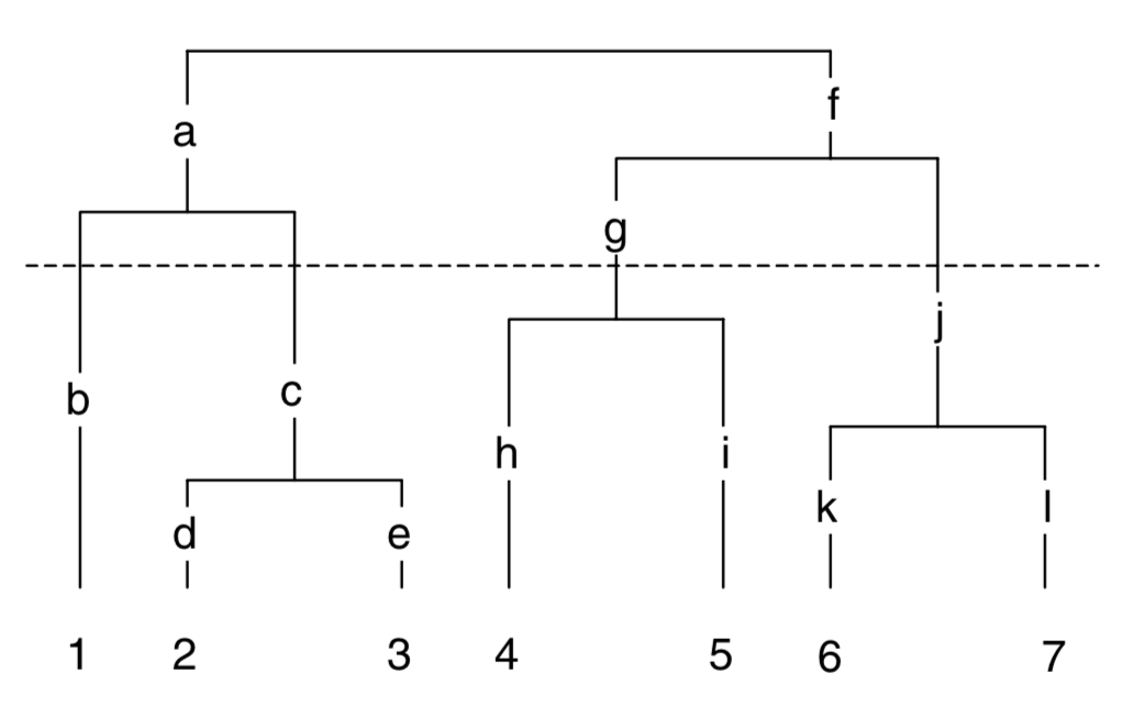
Solution for the genus:species ratio problem = Use phylogenetic trees

Phylodiversity
In the 1990’s conservation biologists recognized the biodiversity is not only species diversity
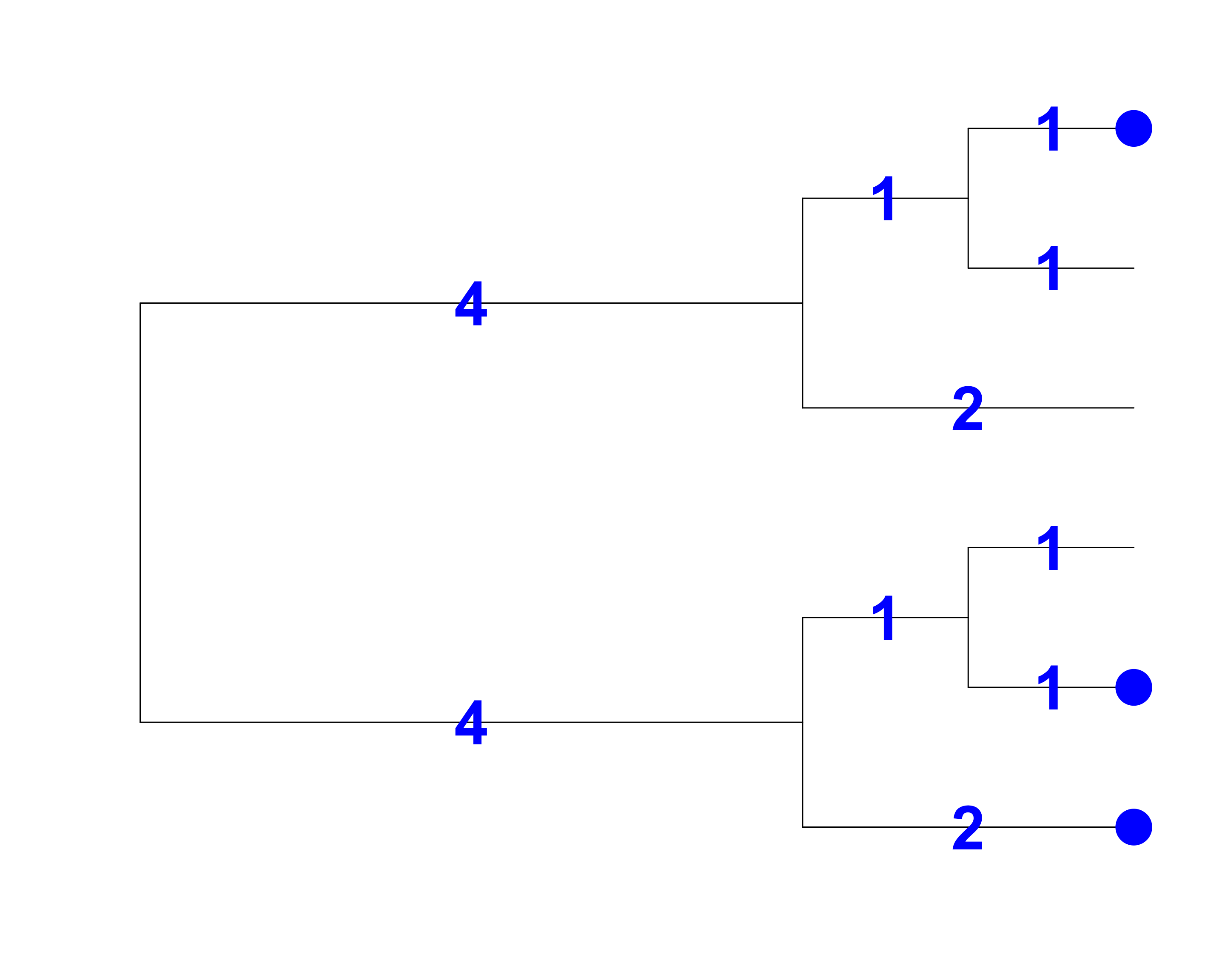
- Biodiversity has several axes or dimensions including genetic, taxonomic, phylogenetic and functional diversity
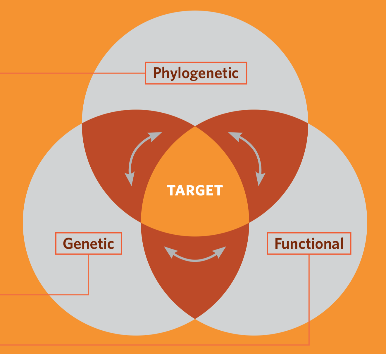
Faith’s Index (PD)
- Total branch length = 18
- PD is the sum of the lengths of all those branches that are members of the corresponding minimum spanning path
- PD is the phylogenetic analogue of taxon richness and is expressed as the number of tree units which are found in a sample
- PD will correlate with species richness
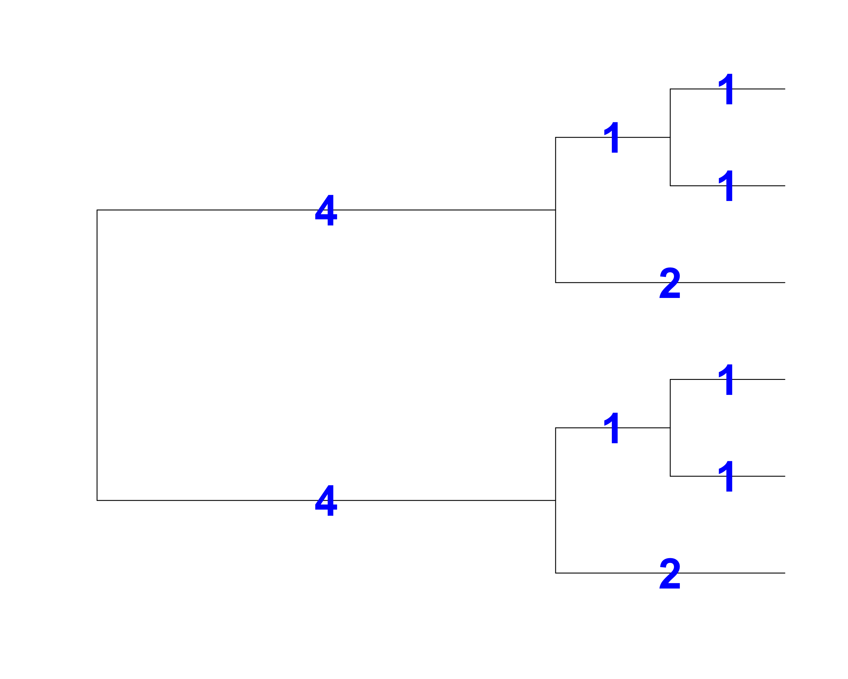
Faith’s Index (PD)
- Total branch length = 9
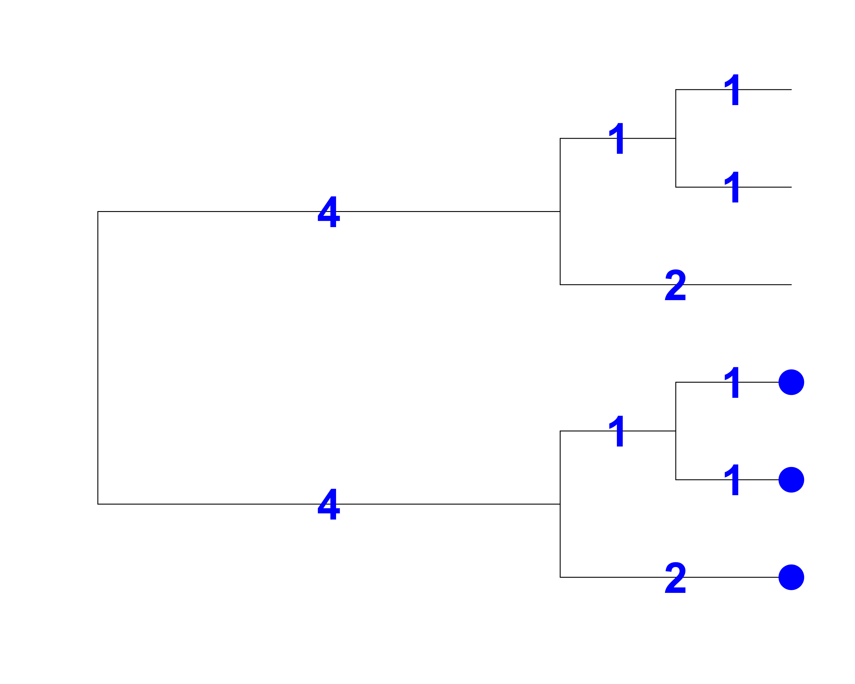
Faith’s Index (PD)
- Total branch length = 14
Petchey’s functional diversity (FD)
- FD is proposed by Owen Petchey in 2002
- FD is the total branch length of the functional dendrogram.
- Analogous to PD
Beyond Faith’s Index (PD)
Solution for genus:species = Use phylogenetic trees to estimate the relatedness of coexisting species
- This solution was first proposed by Cam Webb in 2000

Distance matrix
    A B C D E
  B 1
  C 2 2
  D 4 4 3
  E 5 5 4 2
  F 5 5 4 2 1
Mean Pairwise Distance (MPD) and Net Related Index (NRI)
Let’s consider greatest possible mean pairwise node distance (MPD) for a community of 4 taxa
    A B C D E
  B 1
  C 2 2
  D 4 4 3
  E 5 5 4 2
  F 5 5 4 2 1
A B E
B 1
E 5 5
F 5 5 1Greatest MPD for a community of 4 taxa: 22 / 6 pairs = 3.66 (A, B, E, F)
Mean Nearest Nodal Distance (MNTD) and Nearest Taxa Index (NTI)
Greatest possible nearest nodal distance for a community of 4 taxa = 2 (A, C, D, F; A to C = 2, D to F = 2)
    A B C D E
  B 1
  C 2 2
  D 4 4 3
  E 5 5 4 2
F 5 5 4 2 1Sparks community phylogeny
Do phylogenetically related species have similar ecological niches?
We are assuming that related species are ecologically similar
Related species sometimes have very different traits and ecological niches (e.g., grass-bush, trunk, trunk-crown, trunk-ground and twig ecomorphs)
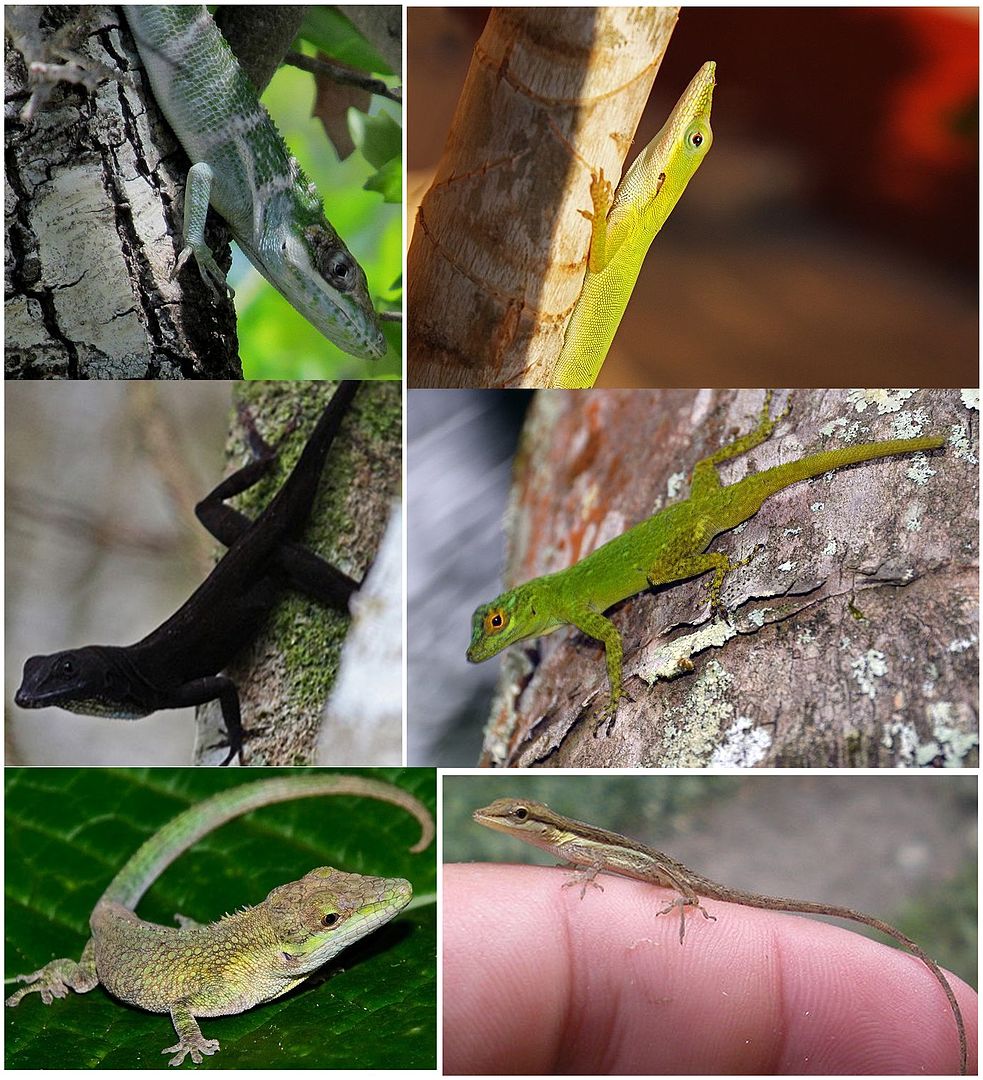
Functional dendrogram vs. phylogeny (Anole example)
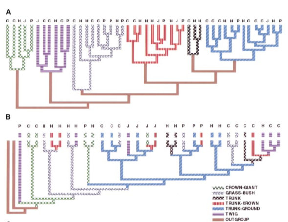
A: Functional dendrogram based on ecomorph
B: Phylogeny indicates frequent evolution of traits
They do not match at all (!!)
Phylogenetically similar = Functional (ecologically) similar??
Putting traits on the tips of phylogeny: phylogenetic signal
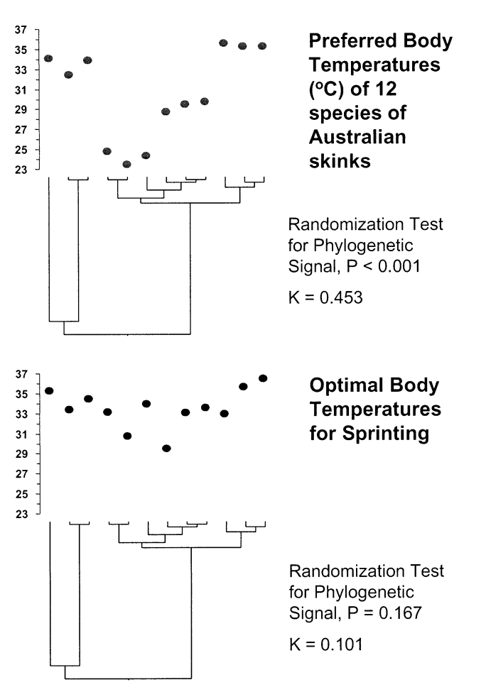
- What is Phylogenetic Signal (K)?
- Phylogenetic signal measures the degree to which related species share similar traits, quantifying the inheritance of traits from either recent or more ancient common ancestors.
- Pagel’s \(\lambda\) is another common measure.
- Interpretation of K Values:
- Large K (phylogenetic conservatism): Trait similarity is high among closely related species, suggesting that traits are conserved across lineages.
- K = 1: Traits are evolving under Brownian motion.
- Small K (phylogenetic divergence): Trait similarity is low among closely related species, indicating that traits have diverged.
- Calculating K:
- K is the ratio of the Mean Squared Error (MSE) of observed trait values to the MSE expected under Brownian motion (random evolutionary change).
Phylogenetic conservatism matters
Phylogenetic conservatism matters
The phylogenetic middleman problem
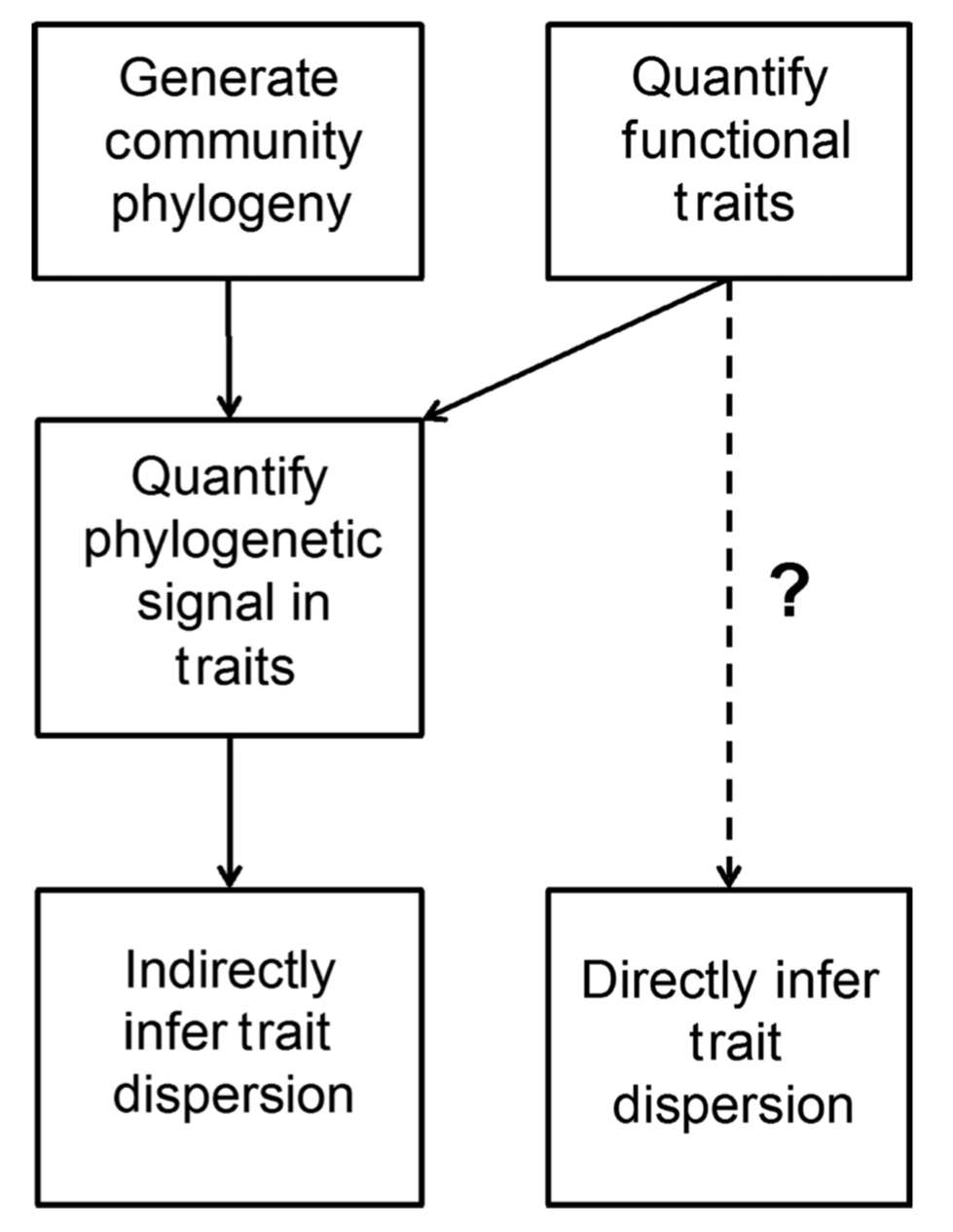
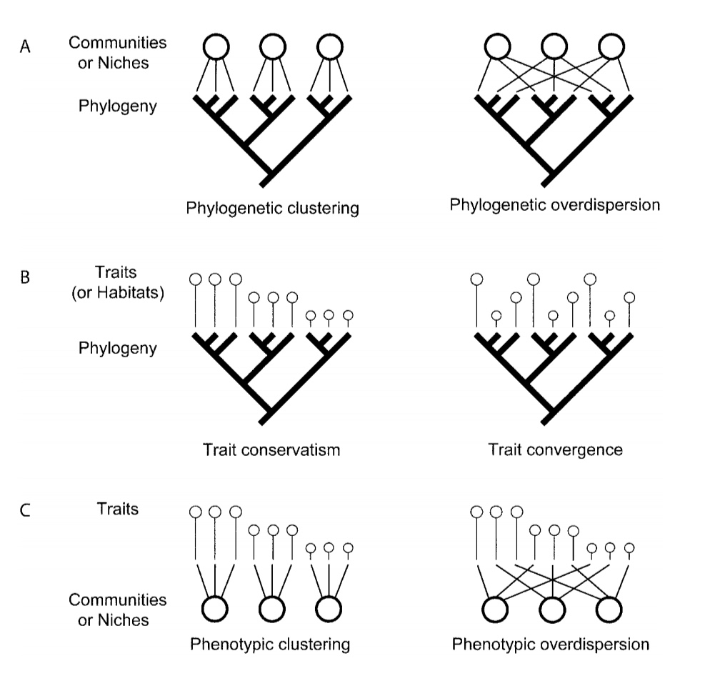
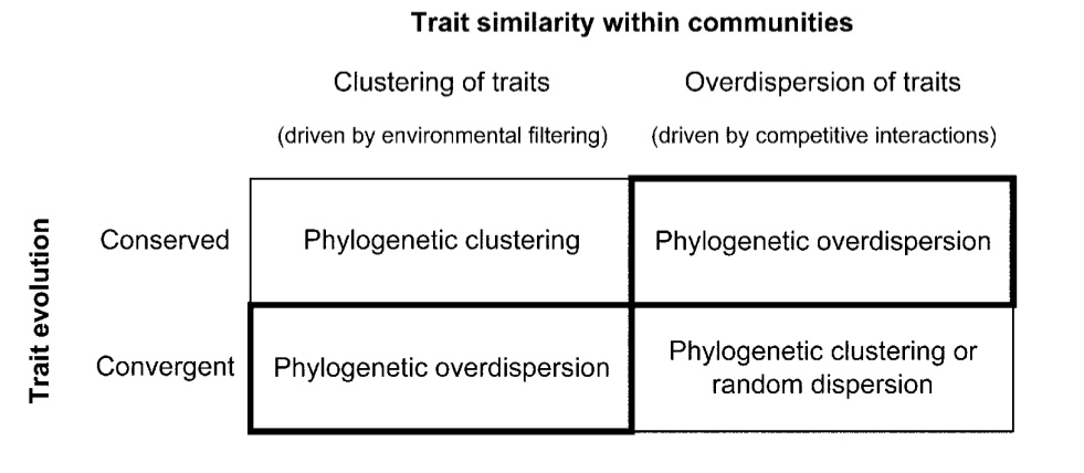
Phylogeny as a proxy for the functional or ecological similarity of species.
Measuring trait data and arraying it on the phylogenetic tree to demonstrate phylogenetic signal in function so that their phylogenetically-based inferences could be supported.
Compared to simply measuring the trait dispersion, this approach is very indirect.
This approach should be avoided! (phylogeny and traits are useful to make meaningful evolutionary inferences)
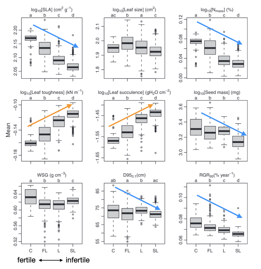
Plant functional traits
Measurable properties of plants that are indicative of ecological strategies
“Hard” traits: e.g., Photosynthetic rates

“Soft” traits: e.g., LMA (leaf mass per area)

Leaf Economic Spectrum (LES)
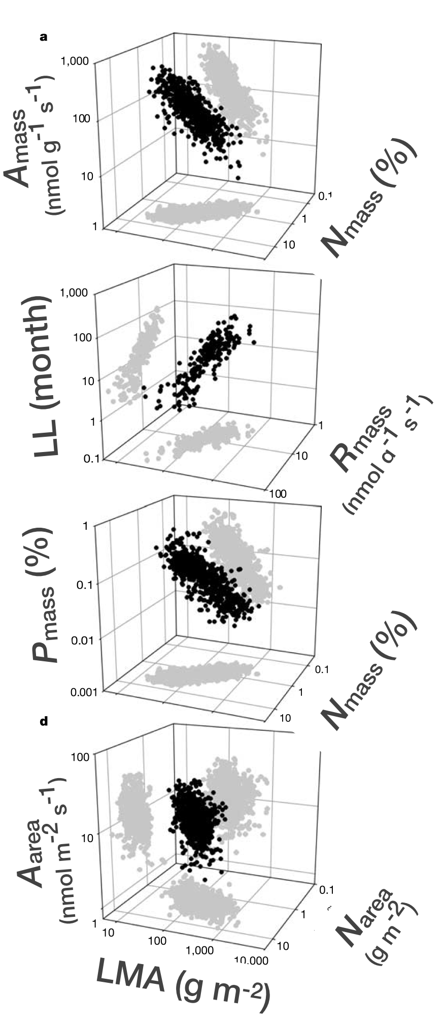
- LES describes pairwise correlations among a bunch of leaf traits from the global leaf database called GLOPNET
- Global leaf function constrained to a single axis (75 % of the variation in the 6 traits)
- Multidimensional (leaf) functional diversity can be mapped into a one-dimensional index
- Controversial because global among‑species patterns don’t always match within‑species or local patterns
Convex hull volume (functional richness)
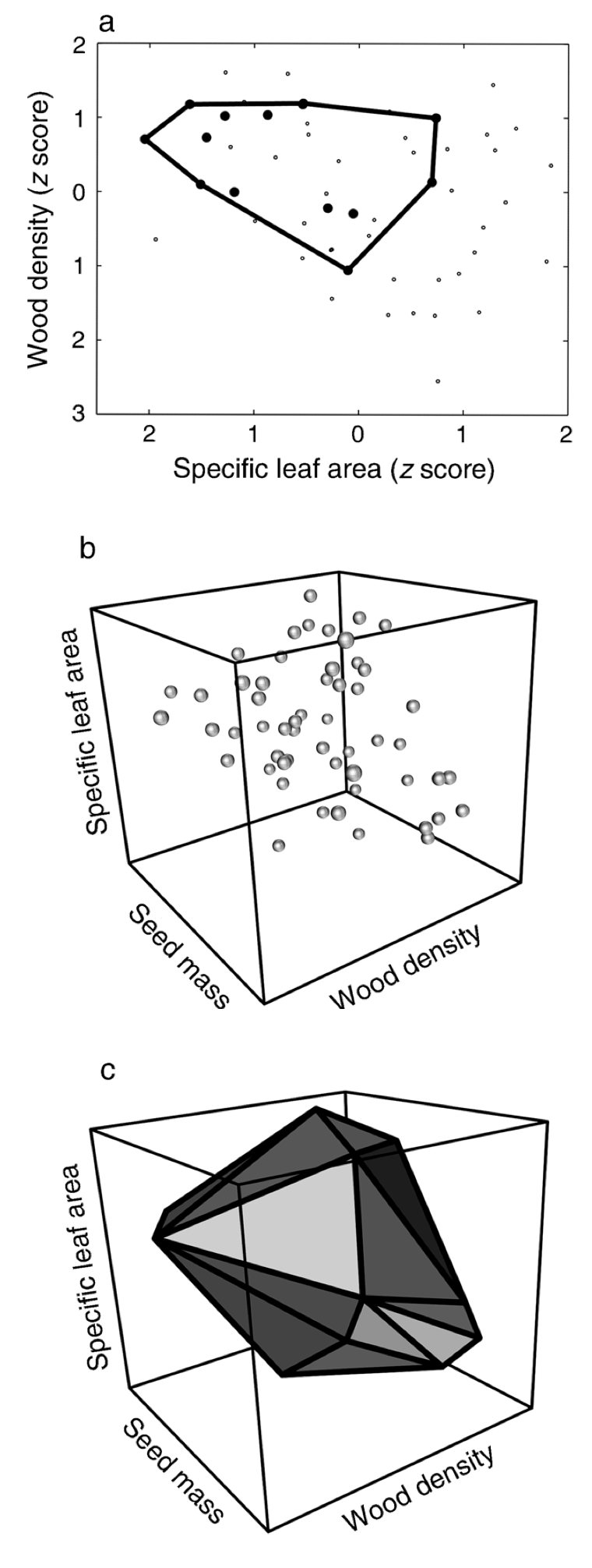
California woody-plant communities (43 plots, 54 species, 3 traits)
Is the trait volume of California woody-plant communities significantly less than expected by chance?
- Environmental filtering
Convex hull volume (functional richness)
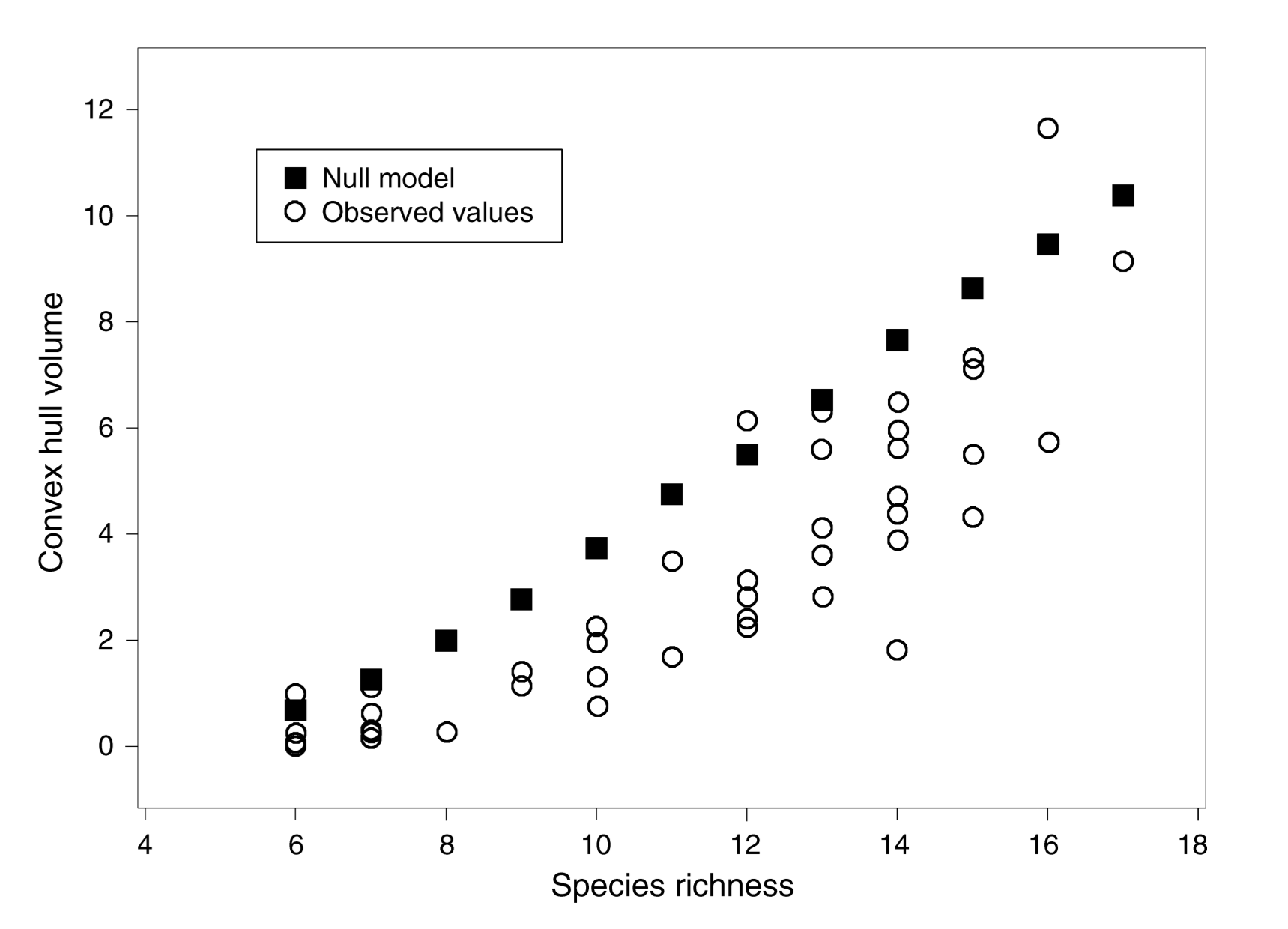
Species in 40 out of 43 plots occupied less trait space than would be expected by chance
Consistent with environmental filtering
Community assembly and trait distribution
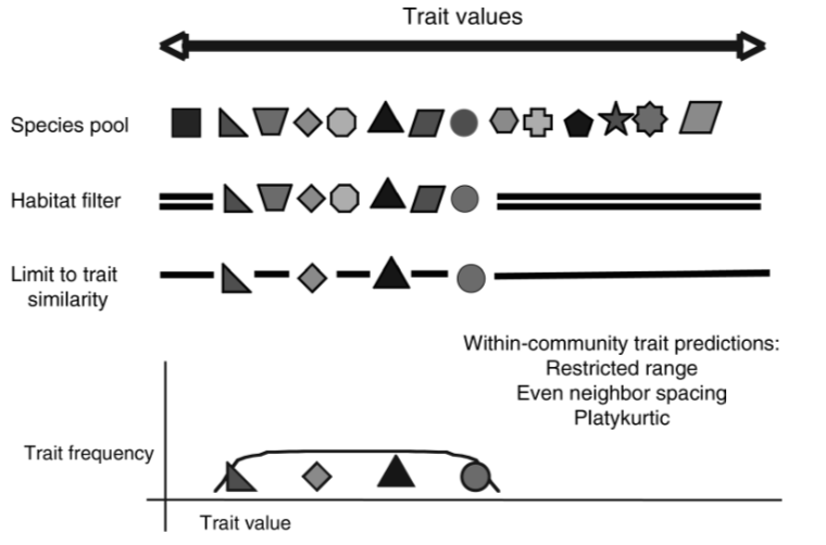
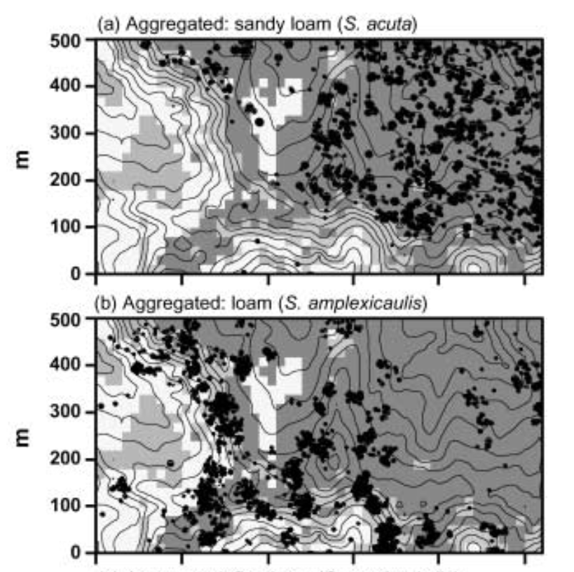
Environmental filtering and limiting similarity can occur at the same time
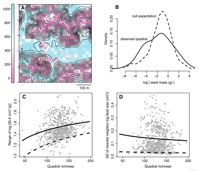
Yasuni tropical tree communities, 25ha, 625 20m x 20m quadrats, 1089 species!
Consistent with environmental filtering
A: Ridgetops have lower than expected SLA and valleys have higher
- Traits match with environmental conditions
B: Seed mass shows broader distribution than expected - Limiting similarity
C: Range of SLA is smaller than expected - Environmental filtering
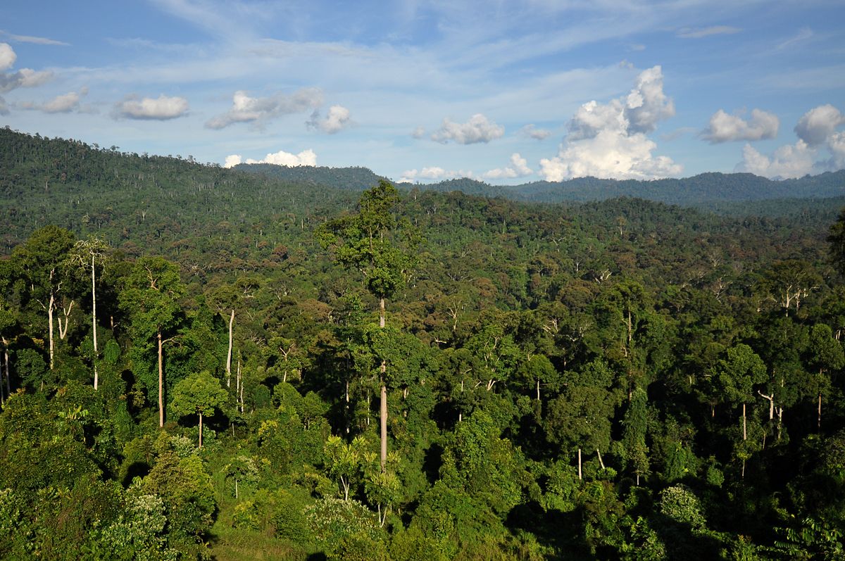
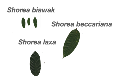
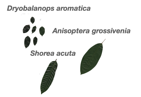
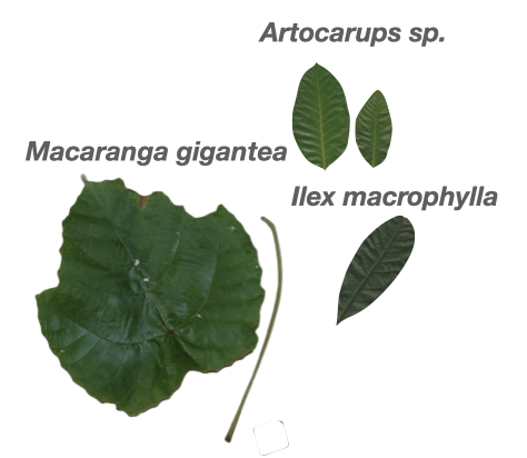
Environmental filtering can occur within dipterocarp trees
Competitive hierarchy

Limiting similarity
Competitive interaction strengths between species will increase with decreasing niche distance, measured as their absolute traits distance \(|t_A - t_B|\)
Competitive hierarchy
Competitive effects of species A on species B will increase with increasing \(t_A - t_B\).
Plant–herbivore interactions
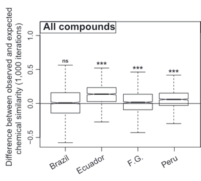
6000+ secondary metabolites from nearly 100 species in a diverse Neotropical plant clade across the whole Amazonia
More differences in their defensive chemistry than expected by chance
Plant–herbivore interactions promote species diversity
Facilitation
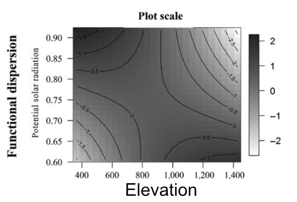
Alpine plants in the Andes
Functional dispersion in harsh environments (higher potential solar radiation)
Facilitation tends to dominate interactions when environmental harshness increases
Trait-based ecology: where are we now?
Community averages can mislead without species‑level context
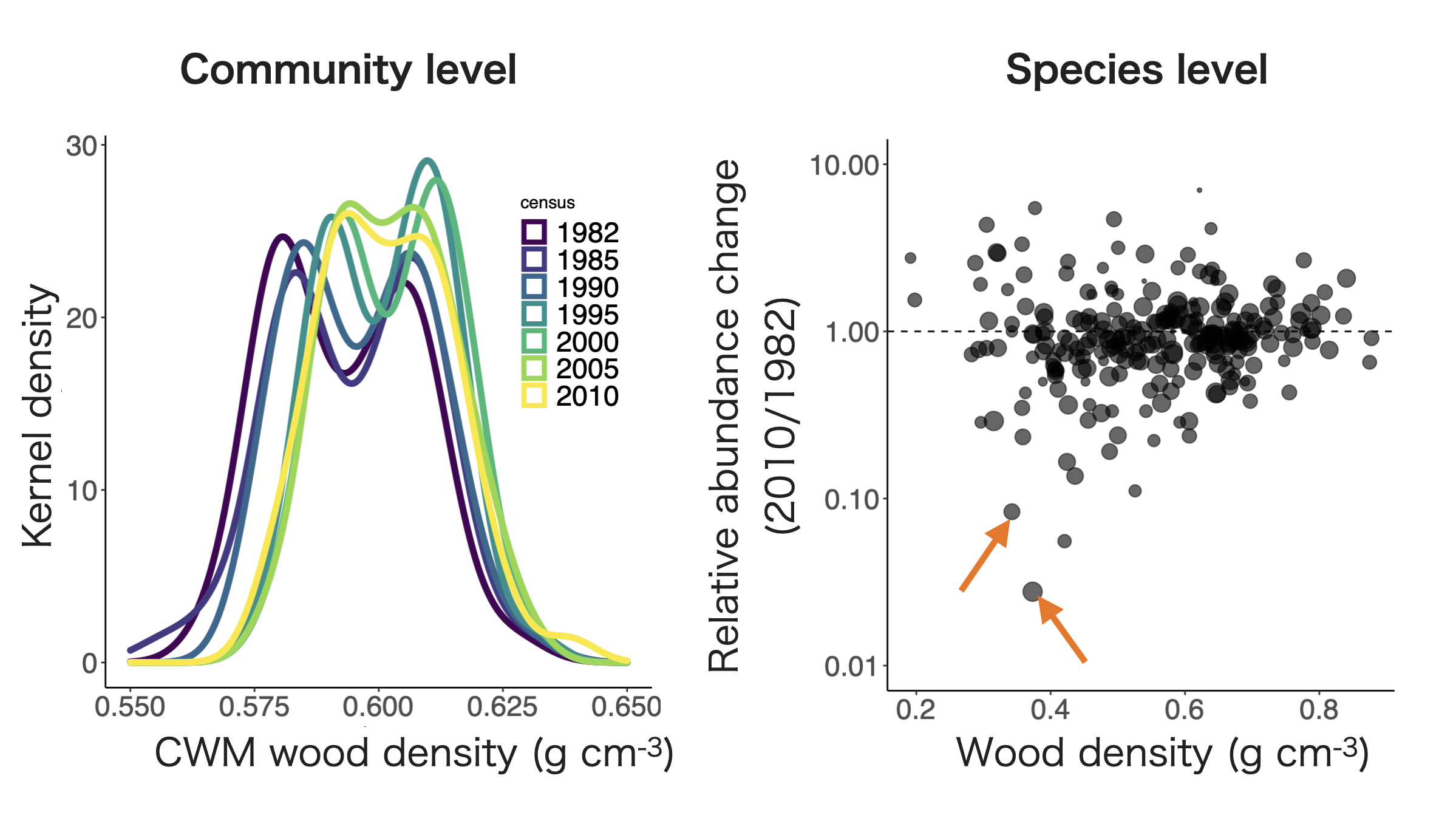
50ha Forest Dynamics Plot on Barro Colorado Island, Panama
CWM wood density trends suggest a community-level response in climate change (i.e, drier conditions).
But 2 of ~300 species (~0.7%) account for ~60% of the temporal shifts in CWM, likely due to species-specific pathogens rather than a community-wide climate response.
Inter‑ and intra‑specific trait patterns often diverge
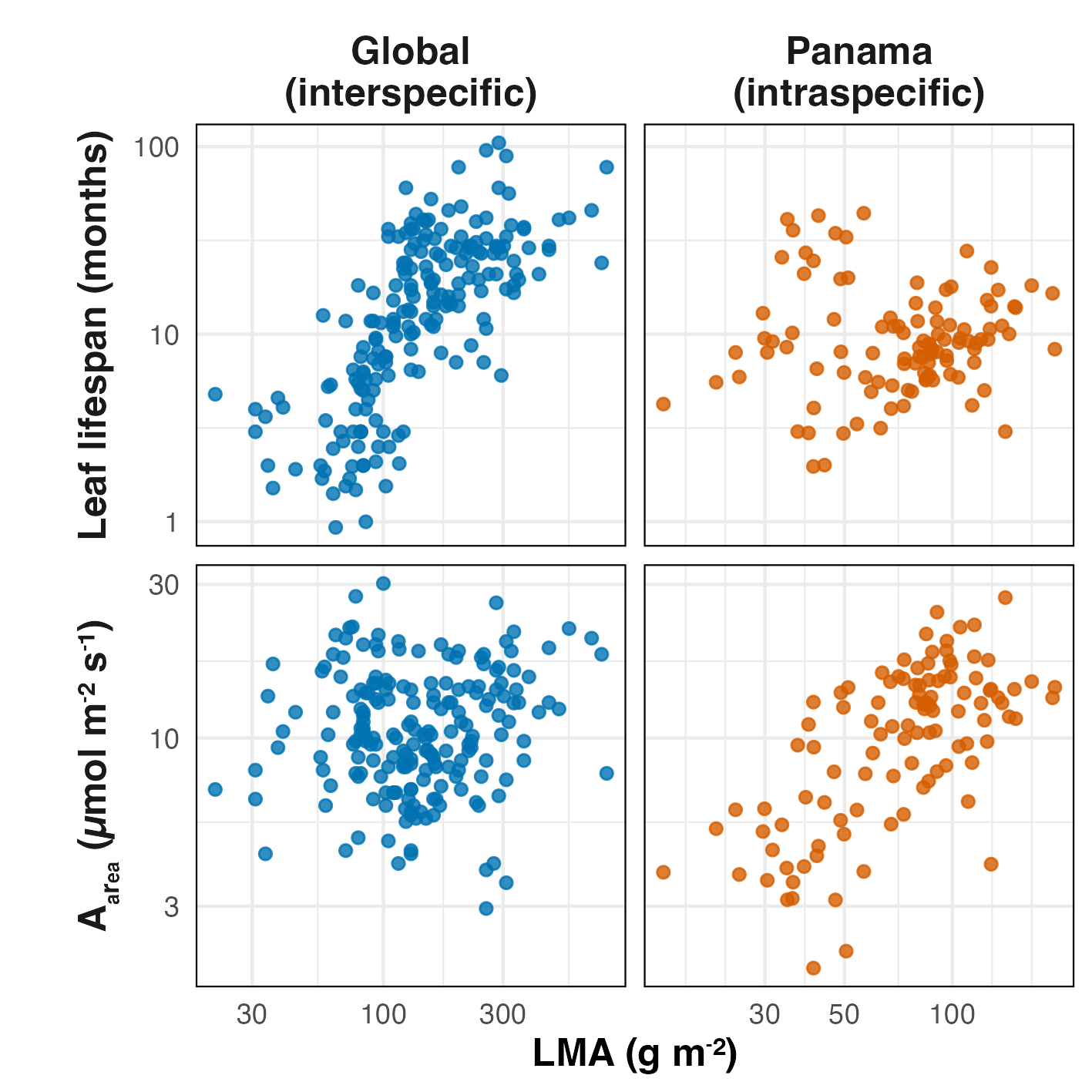
Using harder-to-measure physiological traits may not be enough
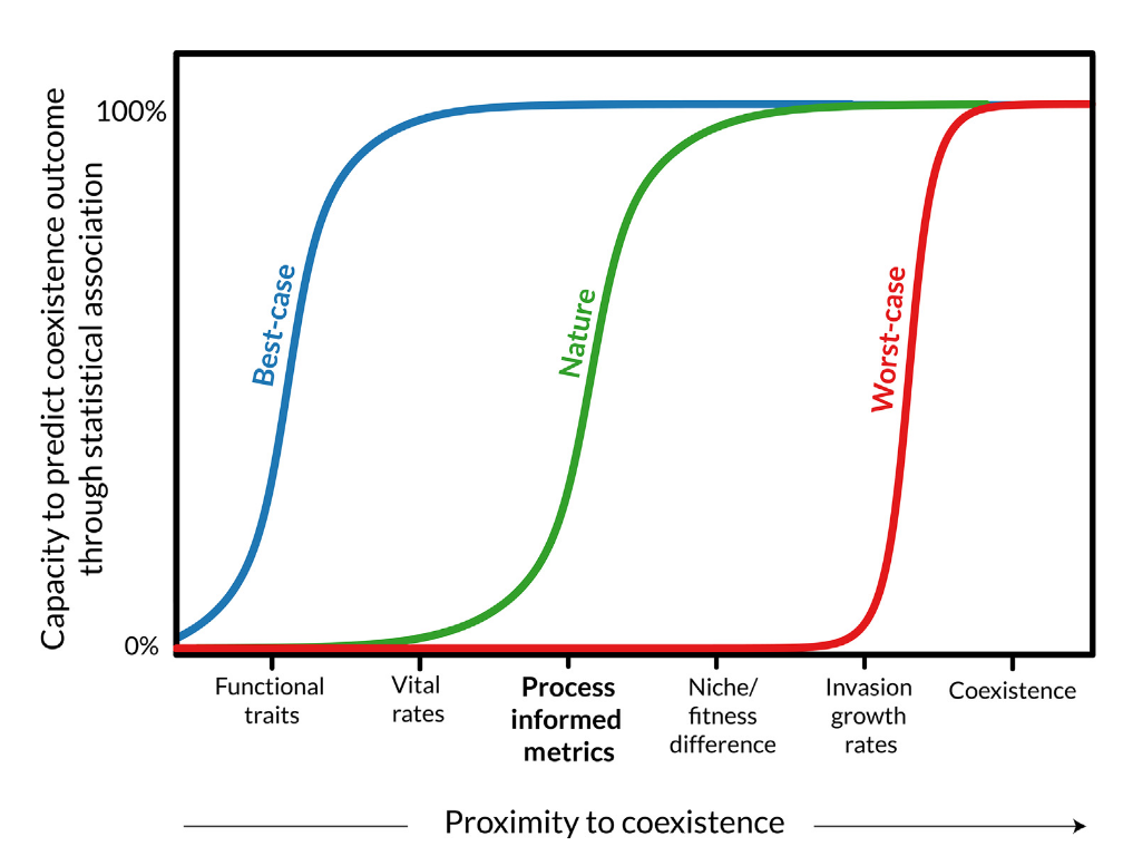
We may need metrics somewhere between functional traits and invasion growth rate (model parameter) to predict coexistence.
Decomposing LMA into metabolic (LMAm) and structural (LMAs) components improves physiological prediction
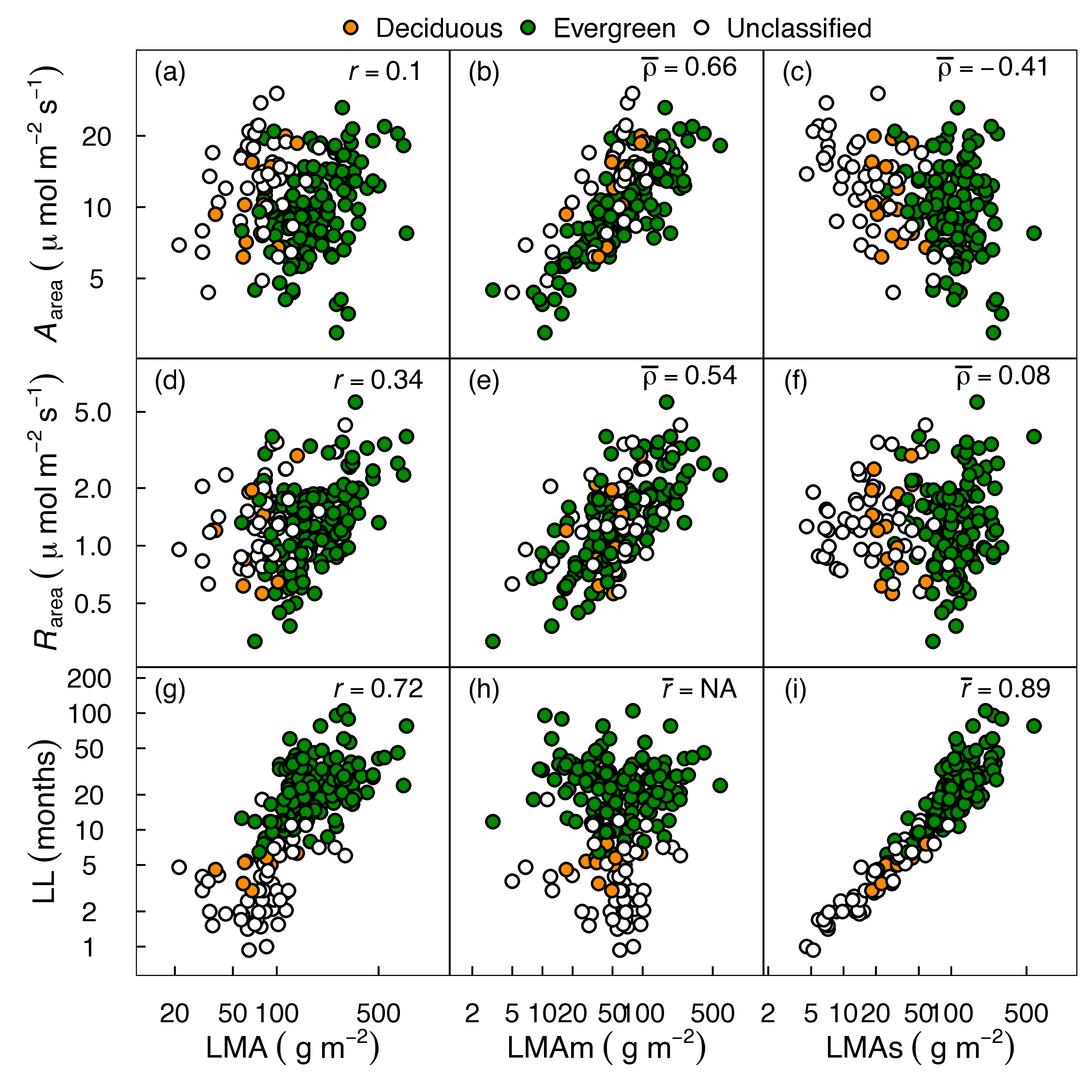
PIMs (LMAm/LMAs) outperform bulk LMA for predicting physiology