Bayesian estimation for ecology
🧑🏻💻 Masatoshi Katabuchi @ XTBG, CAS
- mattocci27@gmail.com
- @mattocci
- github.com/mattocci27/bayes-afec
- https://mattocci27.github.io
November 10, 2024 XTBG AFEC
Objectives
We Learn
Why Bayesian estimation is useful
Why multilevel models are important
We Do Not Learn
- How to use and code Bayesian models in Stan and R
Likelihood
Assuming everyone knows the concept of likelihood
Likelihood and probability density distribution
\(f(x \mid \mu, \sigma) = \frac{1}{\sqrt{2\pi\sigma^2}}\mathrm{exp} \bigl[{-\frac{1}{2}\bigl\{\frac{x-\mu}{\sigma}}\bigr\}^2\bigr]\)
A likelihood function is a probability function that shows how likely it is to observe the data for a specific set of parameters.
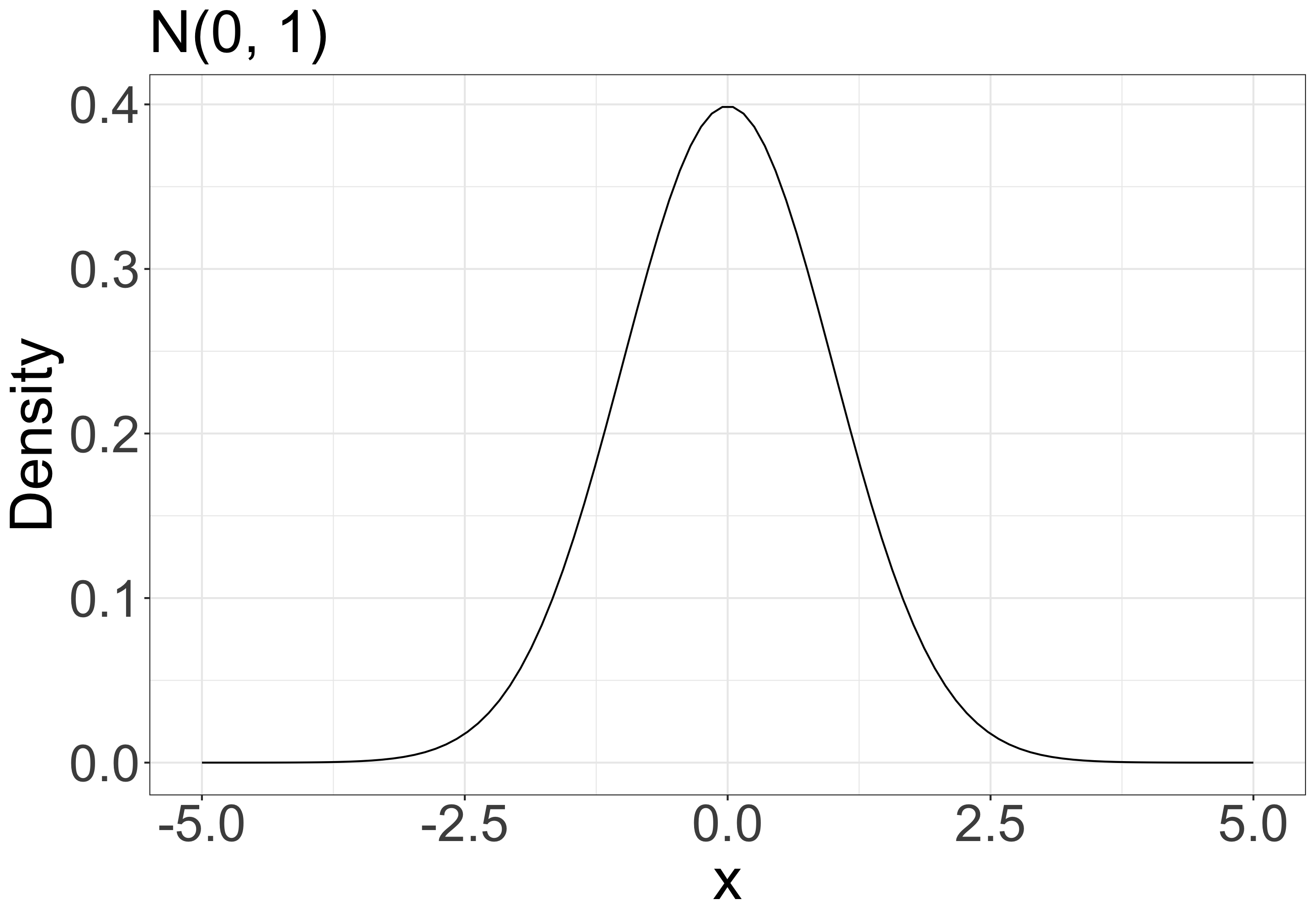
e.g., when your model is \(x \sim \mathcal{N}(\mu = 0, \sigma^2 = 1)\) (normal distribution with mean 0 and variance 1), what is the probability density at x = 1.96?
- \(P(x = 1.96 \mid \mu = 0, \sigma = 1)\)
Likelihood
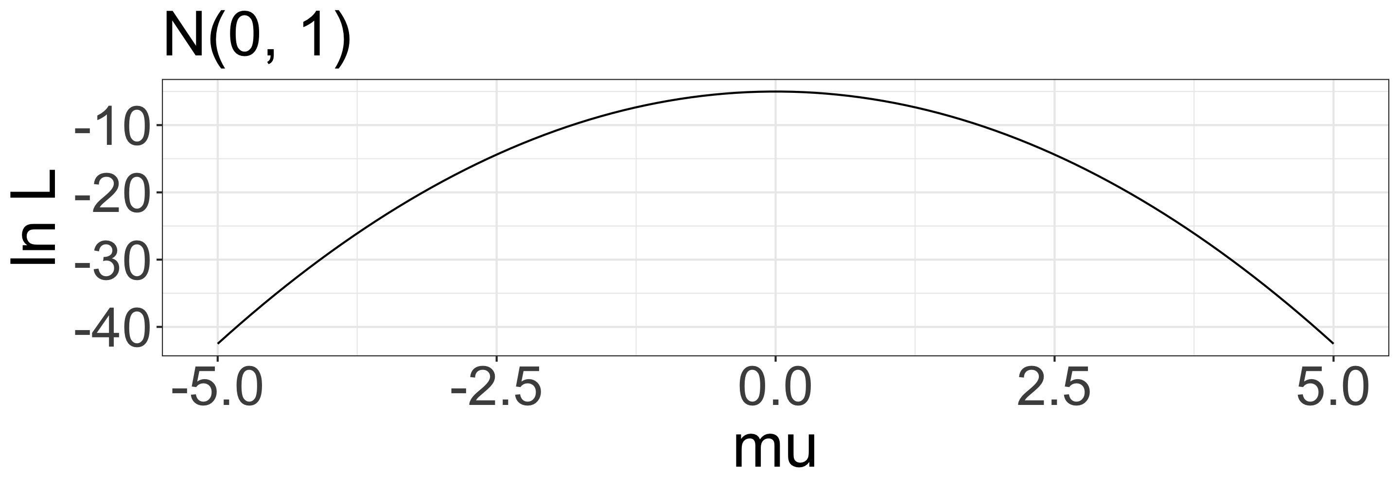
When your data is x = {-1.5, 0, 1.5} and your model is \(x \sim \mathcal{N}(0, 1)\), what is the probability of observing x?
- \(L = P(-1.5 \mid 0, 1) \times P(0 \mid 0, 1) \times P(1.5 \mid 0, 1)\)
- \(\mathrm{ln}\;L = \mathrm{ln}\;P(-1.5 \mid 0, 1) + \mathrm{ln}\;P(0 \mid 0, 1) + \mathrm{ln}\;P(1.5 \mid 0, 1)\)
Likelihood
Because we usually don’t know the true parameters (\(\mu\) and \(\sigma\)), we need to find the parameters that maximize the likelihood function (Maximum Likelihood Estimation).
- e.g., for a liner model \(y = ax + b\), we usually assume that \(y \sim \mathcal{N}(\mu = ax + b, \sigma^2)\), and we want to find the parameters \(a\), \(b\), and \(\sigma\) that maximize the likelihood function: \(P(y \mid ax + b, \sigma)\)
Maximum Likelihood Estimation (MLE)
- 2 survivors out of 5 seedlings: What is the survival probability of seedlings?

\(p\): survival rates, \(1-p\): mortality rate
\(L = {}_5C_2 p^2(1-p)^3\) (Binomial distribution)
\(\mathrm{ln}\;L = \mathrm{ln}\;{}_5C_2 + 2\mathrm{ln}\;p + 3\mathrm{ln}(1-p)\)
\(\frac{d\mathrm{ln}\;L}{dt} = \frac{2}{p} - \frac{3}{1-p} = 0\)
\(p = \frac{2}{5}\)
Outline
Multilevel Model
Conditional Probability and Bayes’s Theorem
Prior
Multilevel Model Revisited
Multilevel Models

Negative density dependence (NDD)
“…rare species suffered more from the presence of conspecific neighbors than common species did, suggesting that conspecific density dependence shapes species abundances in diverse communities.”
- Comita et al. 2010 -
[1] Comita, L. S., Muller-Landau, H. C., Aguilar, S. & Hubbell, S. P. Asymmetric density dependence shapes species abundances in a tropical tree community. Science 329, 330–2 (2010).
Multilevel model (NDD: verbal model)
Inspired by [1] Comita, L. S., Muller-Landau, H. C., Aguilar, S. & Hubbell, S. P. Asymmetric density dependence shapes species abundances in a tropical tree community. Science 329, 330–2 (2010).
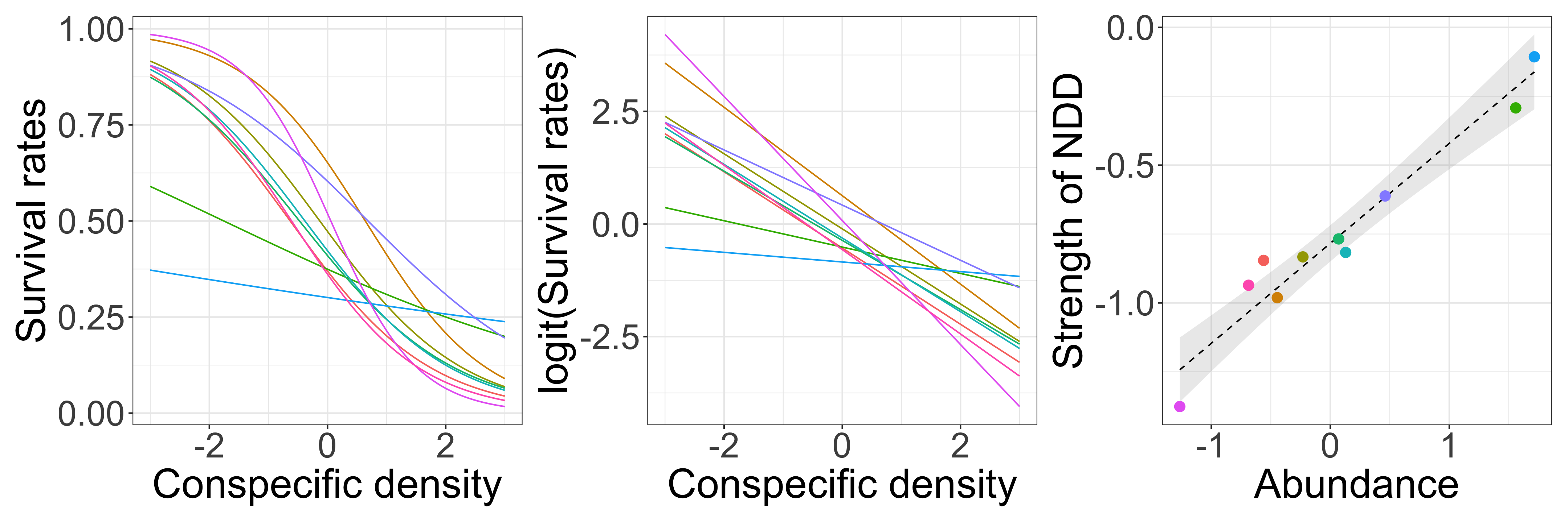
There is negative density dependence (NDD) of seedling survival rate, and the strength of NDD varies among species. The strength of NDD depends on species abundance.
- Model survival rates as a function of conspecific seedling density (individual-level).
- Model the strength of NDD (i.e., slopes) as a function of species abundance (group-level).
Multilevel model (tree allometry: verbal model)
Inspired by [1] Martínez Cano et al. Tropical Tree Height and Crown Allometries for the Barro Colorado Nature Monument, Panama: A Comparison of Alternative Hierarchical Models Incorporating Interspecific Variation in Relation to Life History Traits. Biogeosciences 16, 847–62 (2019).
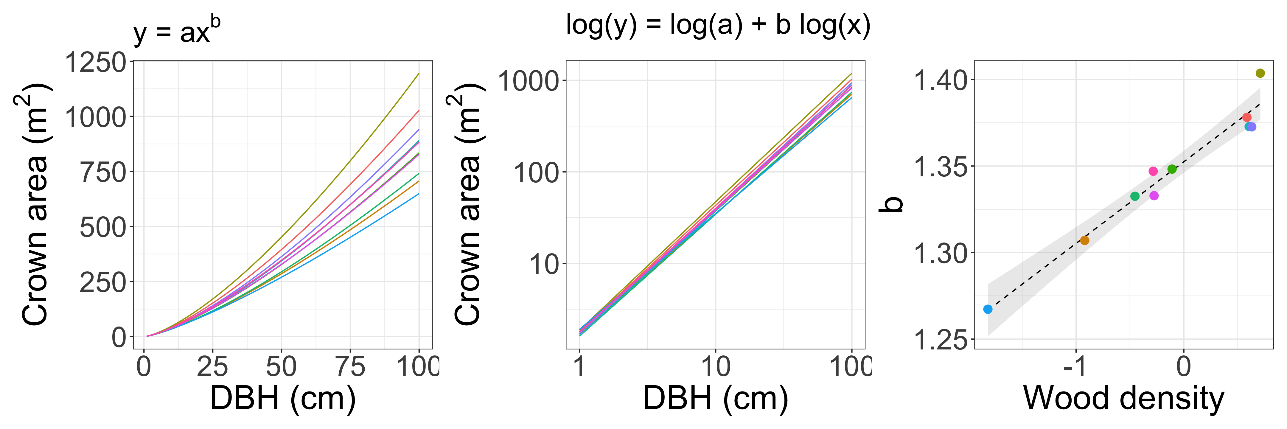
There is a power-law relationship (\(y = ax^b\)) between tree diameter (DBH) and crown area, and the power-law exponent varies among species. Those relationships depend on wood density.
Model crown area as a function of DBH (individual-level).
Model the coefficient b as a function of wood density (group-level).
Multilevel model (MLE: non-verbal ‘dummy’ model 1)
Individual-level model: GLMM
We need to extract the slope coefficients for each species from fit_ind and make new_data.
- This method have low statistical power
Multilevel model (MLE: non-verbal ‘dummy’ model 2)
- This doesn’t work for complicated models
Multilevel model (Bayes: non-verbal model) 🤢
Inspired by [1] Comita, L. S., Muller-Landau, H. C., Aguilar, S. & Hubbell, S. P. Asymmetric density dependence shapes species abundances in a tropical tree community. Science 329, 330–2 (2010).
data{
  int<lower=1> N; // number of samples
  int<lower=1> J; // number of sp
  int<lower=1> K; // number of tree-level preditors (i.e, CONS, HETS,...)
  int<lower=1> L; // number of sp-level predictors (i.e., interecept, SLA,...)
  matrix[N, K] x; // tree-level predictor
  matrix[L, J] u; // sp-level predictor
  array[N] int<lower=0, upper=1> suv; // 1 or 0
  array[N] int<lower=1, upper=J> sp; // integer
}

parameters{
  matrix[K, L] gamma;
  matrix[K, J] z;
  cholesky_factor_corr[K] L_Omega;
  vector<lower=0, upper=pi() / 2>[K] tau_unif;
}

transformed parameters{
  matrix[K, J] beta;
  vector<lower=0>[K] tau;
  for (k in 1:K) tau[k] = 2.5 * tan(tau_unif[k]);
  beta = gamma * u + diag_pre_multiply(tau, L_Omega) * z;
}

model {
  vector[N] mu;
  to_vector(z) ~ std_normal();
  L_Omega ~ lkj_corr_cholesky(2);
  to_vector(gamma) ~ normal(0, 2.5);
  for (n in 1:N) {
    mu[n] = x[n, ] * beta[, sp[n]];
  }
  suv ~ bernoulli_logit(mu);
}

generated quantities {
  vector[N] log_lik;
  corr_matrix[K] Omega;
  Omega = multiply_lower_tri_self_transpose(L_Omega);
  for (n in 1:N) {
    log_lik[n] = bernoulli_logit_lpmf(suv[n] | x[n, ] * beta[, sp[n]] +
      phi[plot[n]] + xi[census[n]] + psi[tag[n]]);
  }
}
\(s_{i,j} \sim \mathcal{B}(p_{i, j})\): likelihood
\(\mathrm{logit}(p_{i,j}) = \boldsymbol{x_{i}} \cdot \boldsymbol{\beta_{j}}\): individual-level model
\(\boldsymbol{\beta_j} = \boldsymbol{\gamma_k} \cdot \boldsymbol{u_j} + \mathrm{diag}(\boldsymbol{\sigma})\cdot \boldsymbol{L} \cdot \boldsymbol{z}\): species-level model
\(L \sim \mathrm{LkjCholesky}(\eta)\): prior (?)
\(z_j \sim \mathcal{N}(0, 1)\): prior (?)
\(\tau \sim \mathrm{Cauchy}(0, 2.5)\): prior (?)
\(\gamma_k \sim \mathcal{N}(0, 2.5)\): prior (?)
Conditional Probability and Bayes’s Theorem
Conditional Probability and Bayes’s Theorem
\[ P(A \mid B) = \frac{P(B \mid A) \times P(A)}{P(B)} \]
Conditional probability
Bayes’s Theorem
Forward / inverse problems
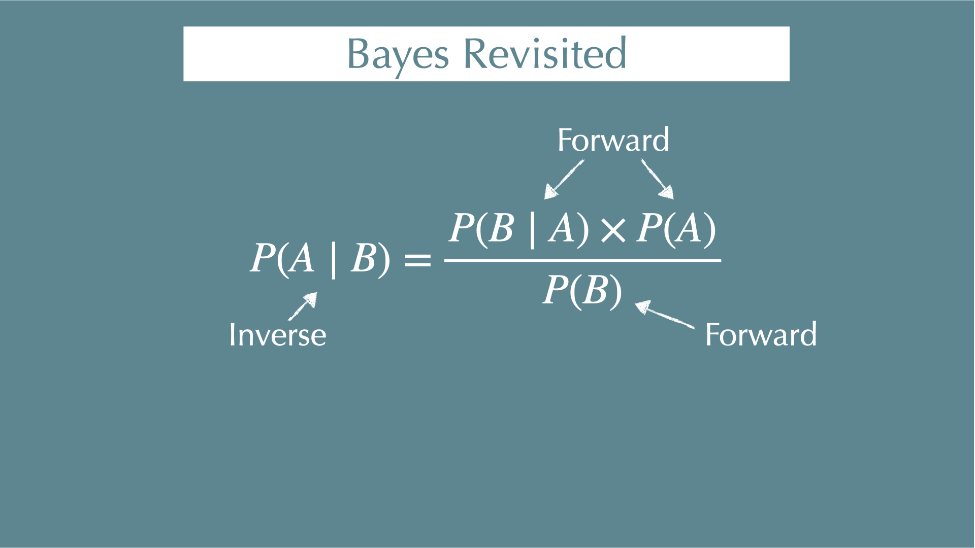
Bayes revisit
Probability

Probility of A:
\[ P(A) = \frac{A}{U} \]
e.g., probability of rolling a dice and getting an odd number is 3/6 = 1/2
Conditional Probability
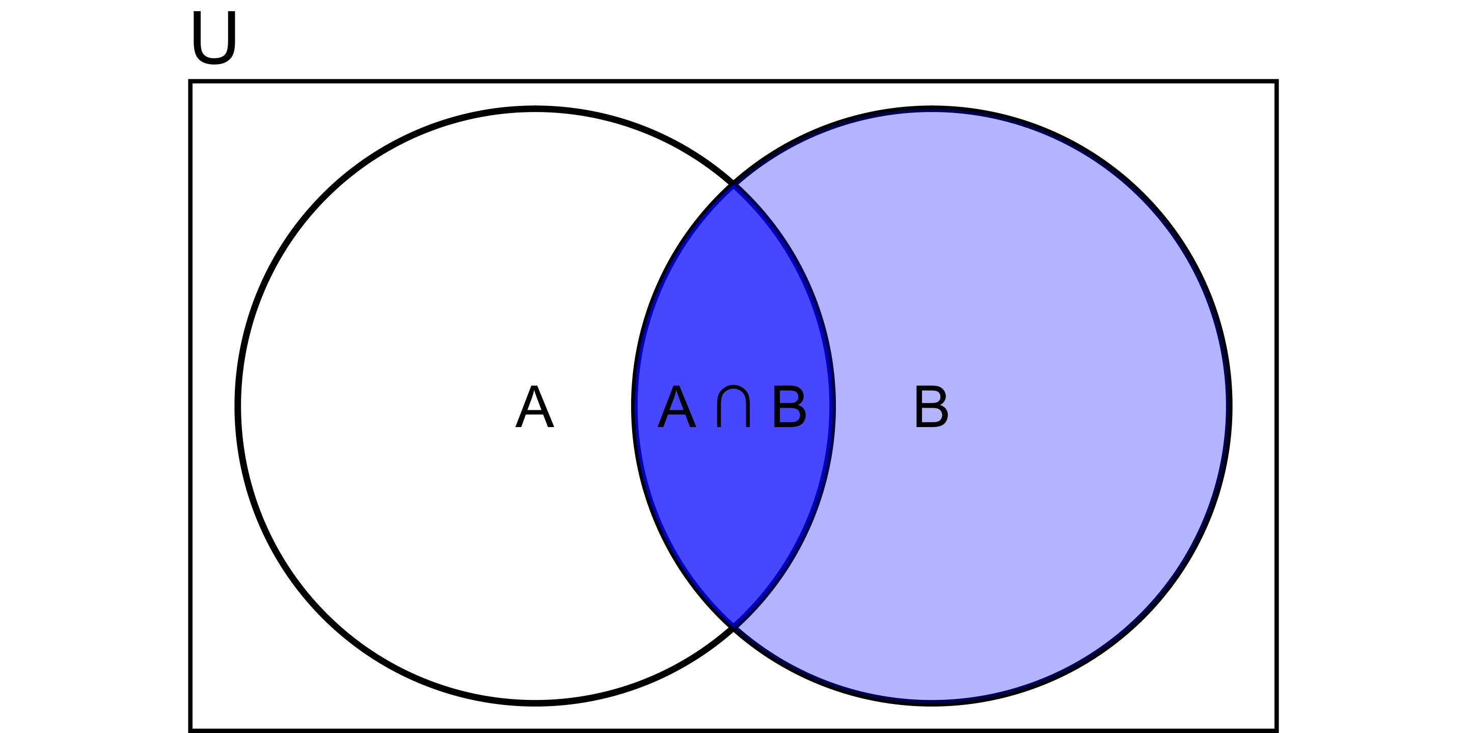
Probability of A occurring given B has already occurred:
\[ P(A \mid B) = \frac{P(A \cap B)}{P(B)} \]
e.g.,
- P(hangover) = 4%
- P(hangover | beer) = 6%.
- P(hangover | baiju) = 85%.
Bayes’s Theorem
\[ P(B \mid A) = \frac{P(A \cap B)}{P(A)} \]
\[ P(A \mid B) = \frac{P(A \cap B)}{P(B)} \]
\[ P(A \mid B) \times P(B) = P(B \mid A) \times P(A) \]
\[ P(A \mid B) = \frac{P(B \mid A) \times P(A)}{P(B)} \]
Why is this useful?
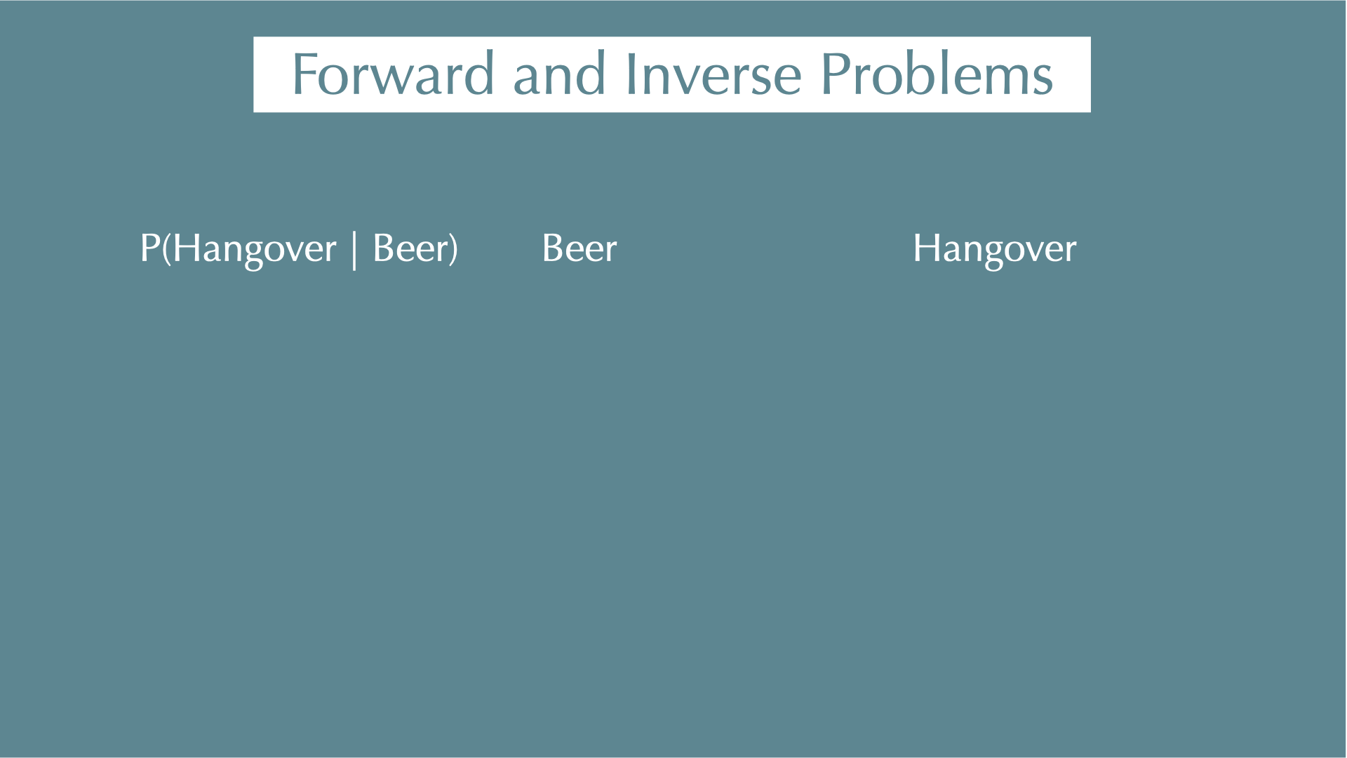
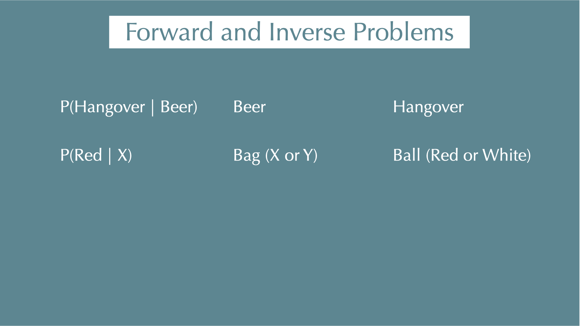
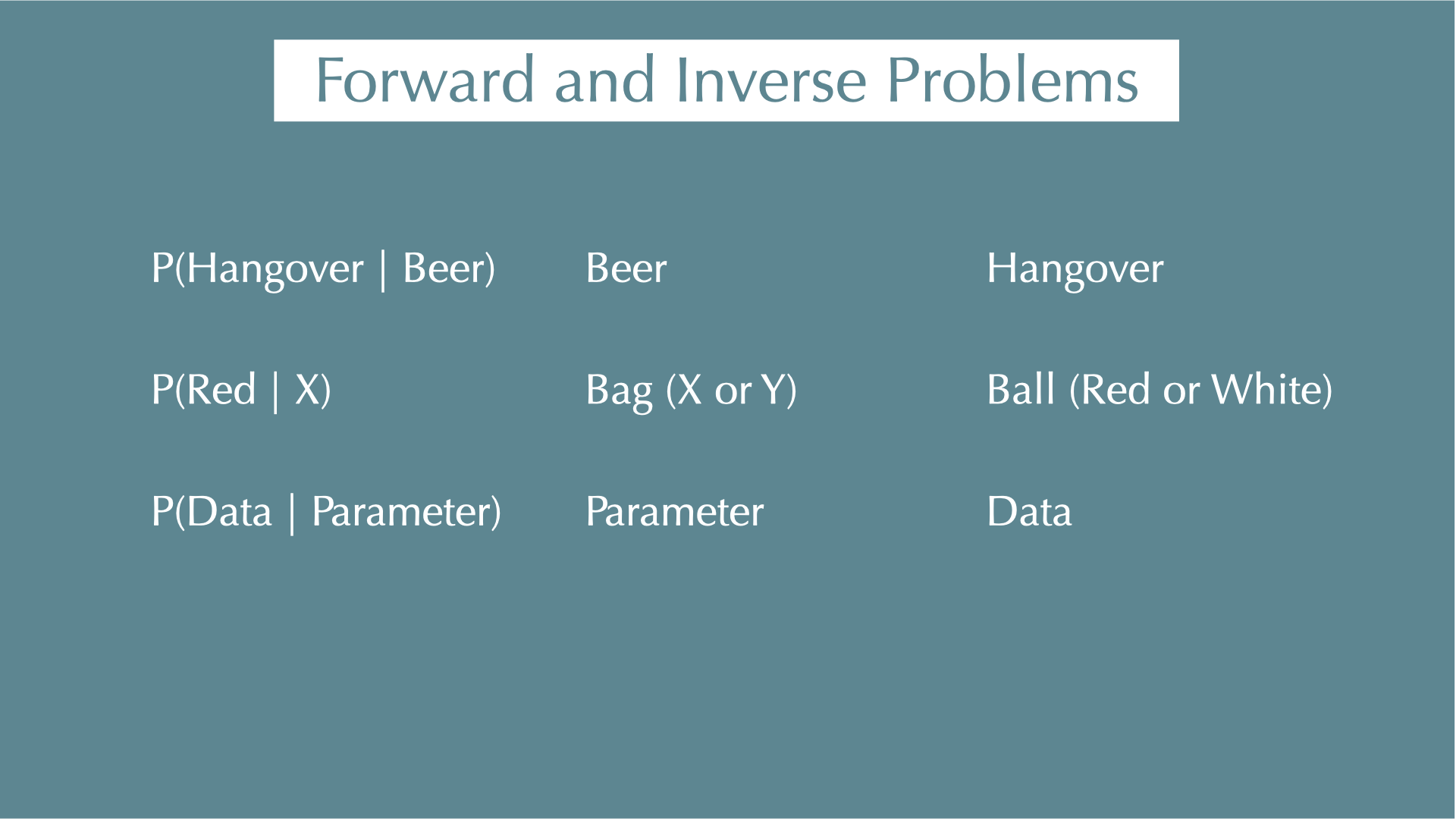
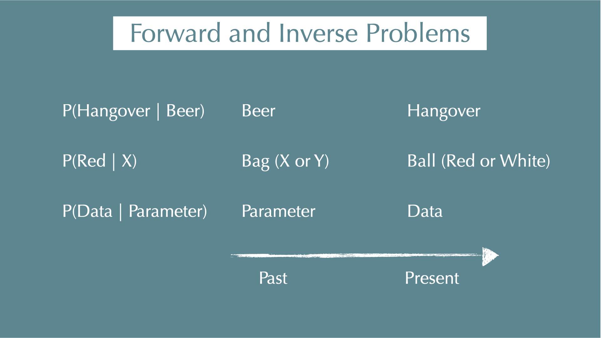
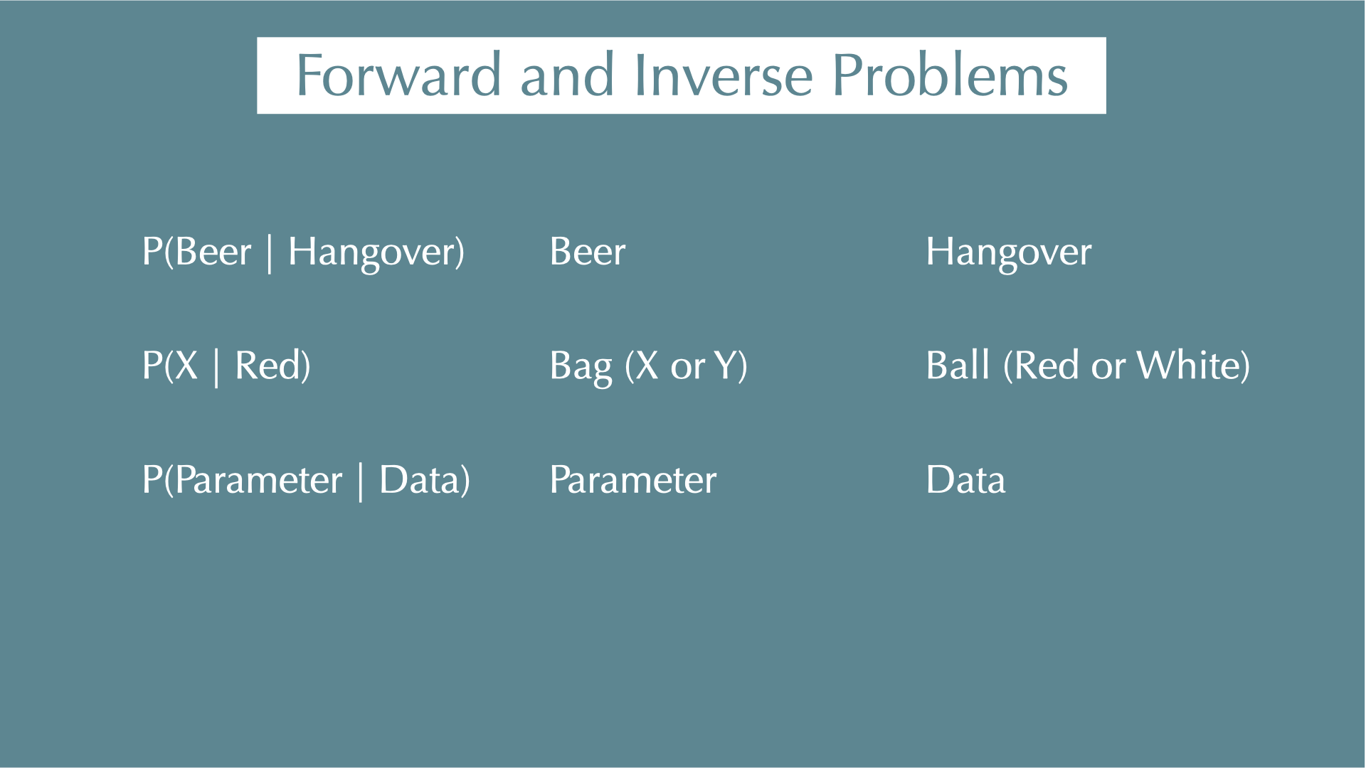
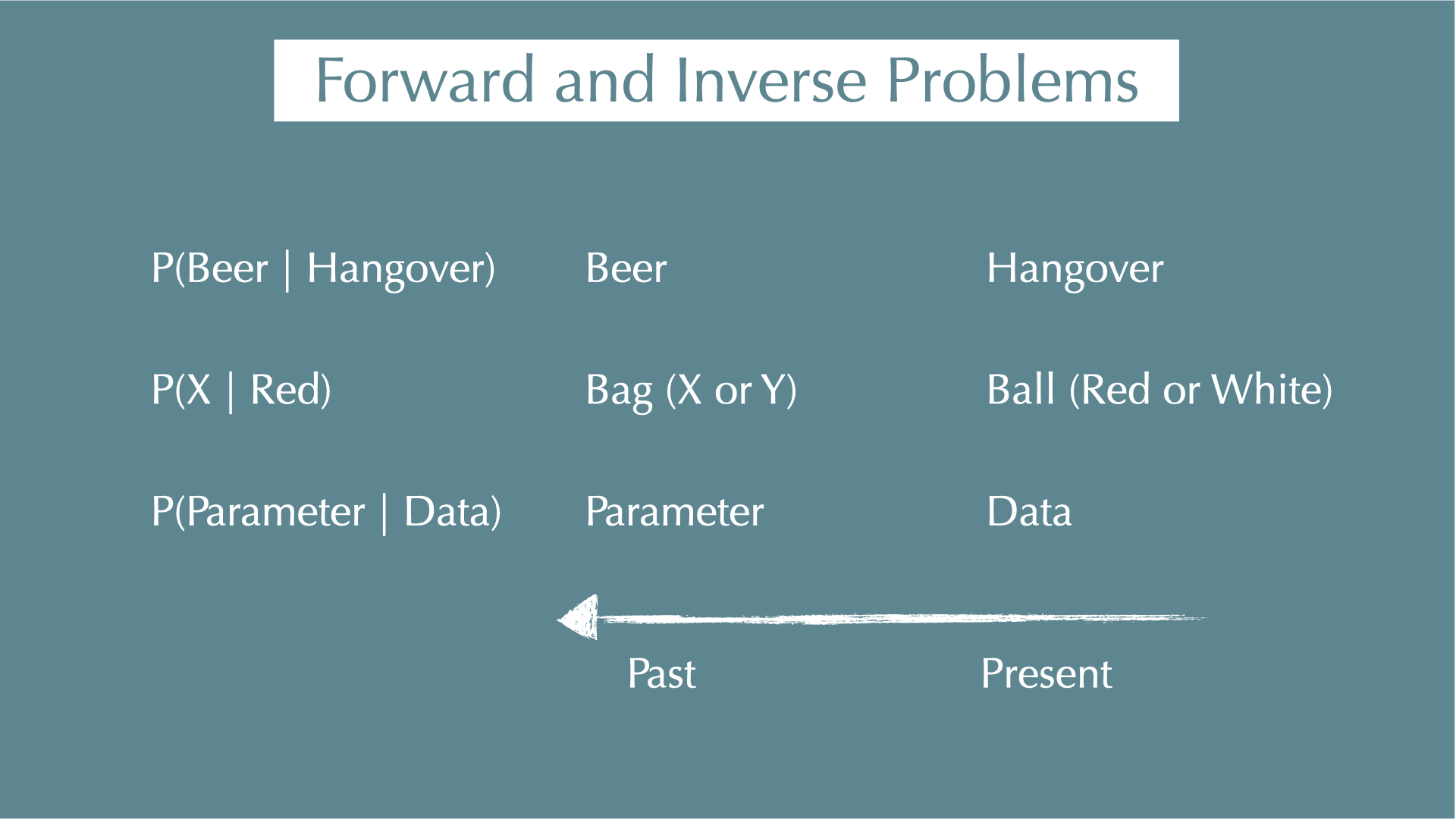
Forward and Inverse Problems
X: 3 red balls, 5 white balls
Y: 1 red balls, 3 white balls
Randomly choose a bag X or Y
\(P(A)\): Choosing X
\(P(B)\): Drawing a red ball
\(P(B \mid A)\): Getting a red ball from X
\(P(A \cap B)\): Choosing X and drawing a red ball
\(P(A \mid B)\): Picked X, because you got a red ball(?)
\(P(A) = 1/2\)
\(P(B \mid A) = 3/8\)
\(P(B)\) = 1/2 \(\times\) 3/8 + 1/2 \(\times\) 1/4 = 5 /16
\(P(A \cap B)\) = 1/2 \(\times\) 3/8 = 3/16
\(P(A \mid B)\) = \(P(A \cap B) / P(B)\) = (3/16) / (5/16) = 3/5
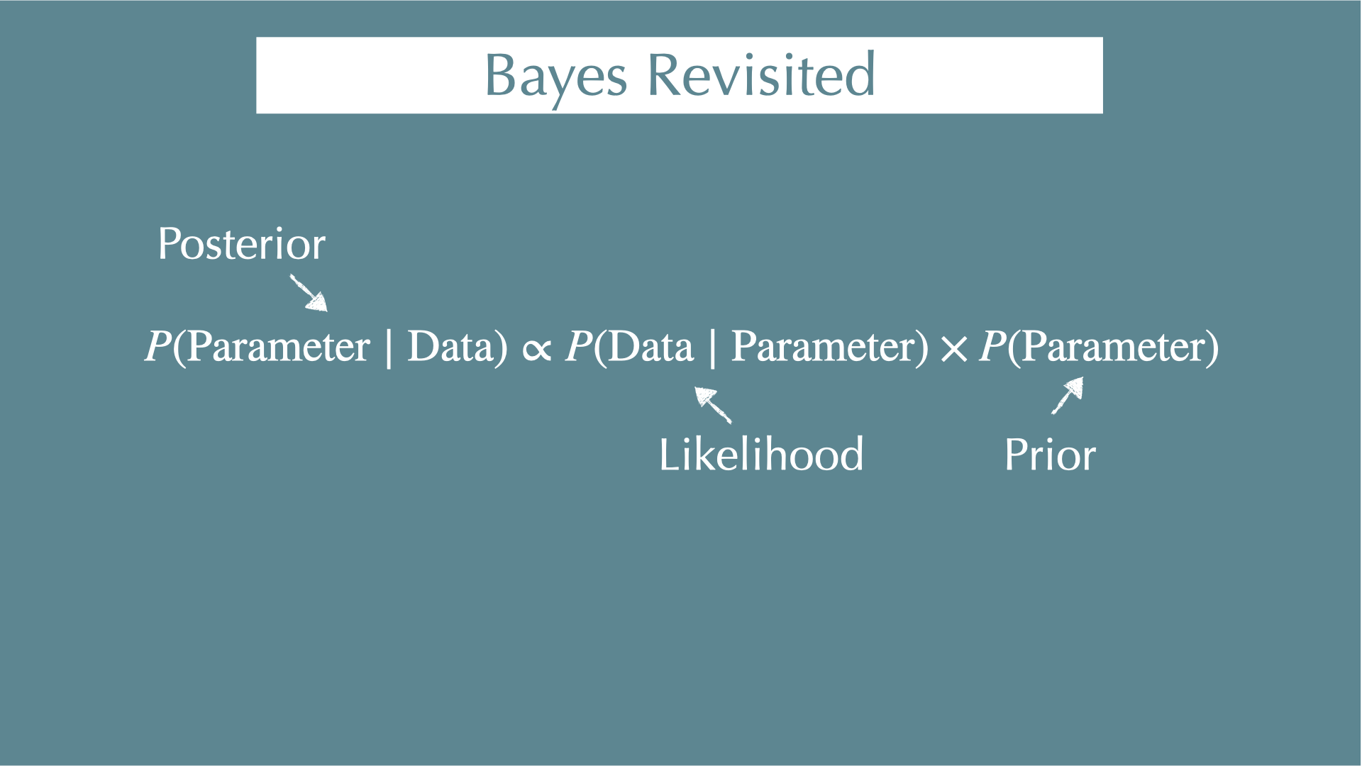
\[ P(\mathrm{Parameter} \mid \mathrm{Data}) = \frac{P(\mathrm{Data} \mid \mathrm{Parameter}) \times P(\mathrm{Parameter})}{P(\mathrm{Data})} \]
\(P(\mathrm{Parameter} \mid \mathrm{Data})\)
- When you got your data, what were the parameters behind the data (e.g., coefficients of regressions)?
\(P(\mathrm{Data} \mid \mathrm{Parameter})\)
- When you know your parameters, what is the probability of getting your data? (i.e., likelihood)
\(P(\mathrm{Parameter})\)
- Probability to get your parameters. This is what you assume for your parameter before you see any data (i.e., prior).
\(P(\mathrm{Data})\)
- Independent with parameters (i.e., constant)
Prior
Prior (coins)
MLE
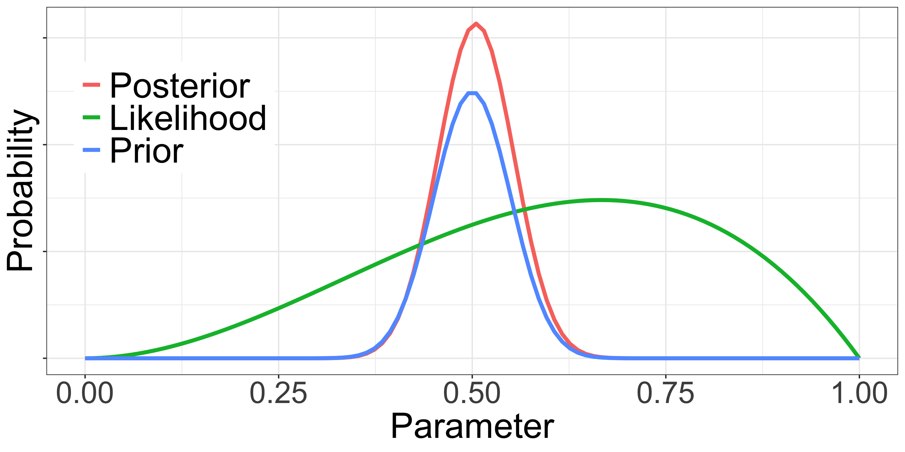
- A: 2 head out of 3 tosses -> 2/3 = 0.666
- B: 60 heads out of 100 tosses -> 60/100 = 0.6
Bayesian
\(L_A = {}_3C_2 p^2 (1-p)^1\)
\(L_B = {}_{100}C_{60} p^{60} (1-p)^{40}\)
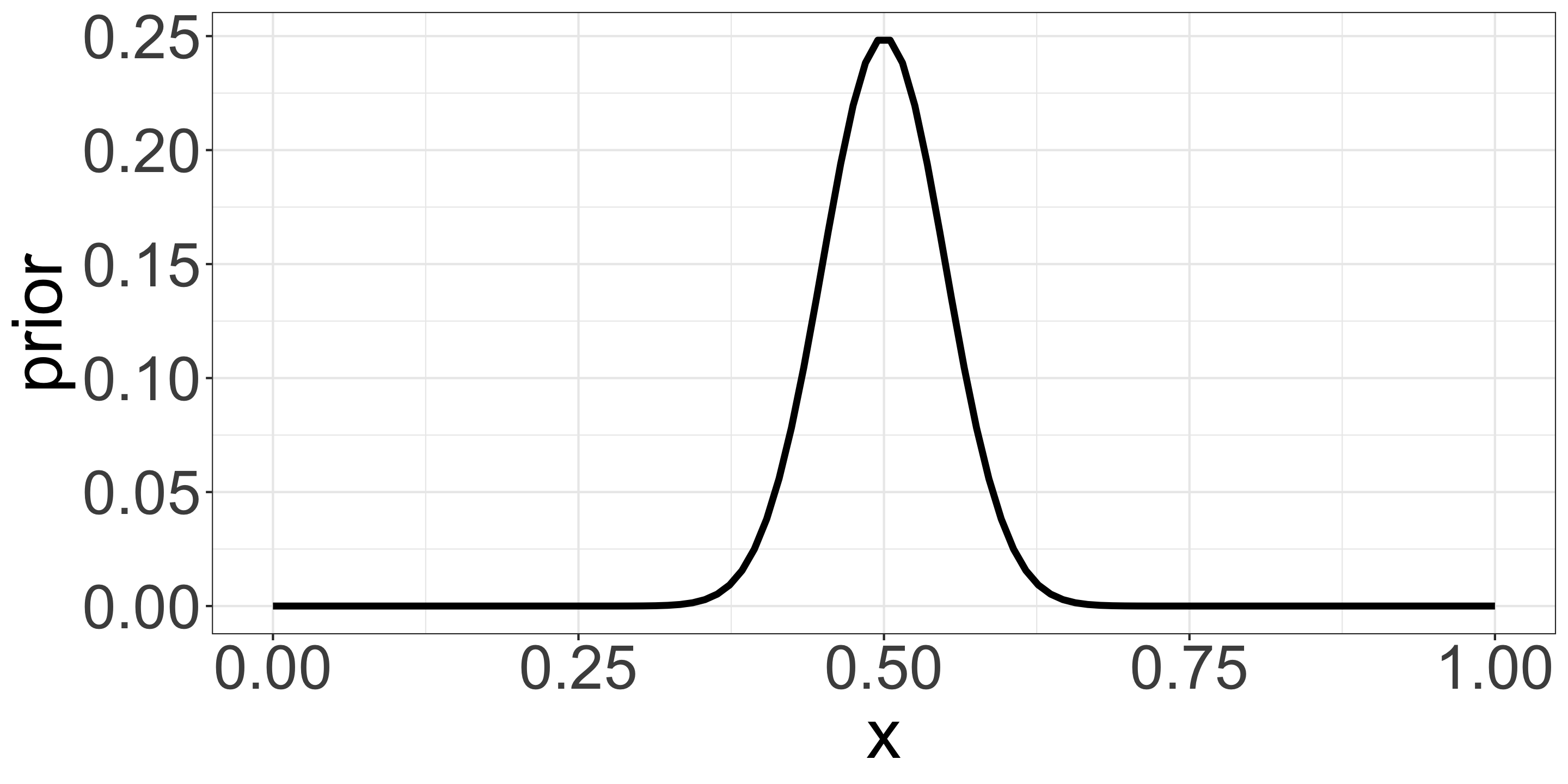
\(\mathrm{Prior} \propto p^{50} (1-p)^{50}\)
- Beta distribution with mean 0.5 and small variance
Prior (coins)
\(Post_A \propto p^2 (1-p)^1 \times p^{50} (1-p)^{50}\)
\(Post_A \propto p^{52} (1-p)^{51}\)
\(Post_A' = 52p^{51}(1-p)^{51}-\) \(51p^{52}(1-p)^{50}\)
p = 52/103 = 0.5048
\(Post_B \propto p^{60} (1-p)^{40} \times p^{50} (1-p)^{50}\)
\(Post_B \propto p^{110} (1-p)^{90}\)
p = 110/200 = 0.55
- \(Like_B\): 60 heads out of 100 tosses
- \(Prior_B\): P(H) is about 50%, a reasonable assumption based on existing knowledge of coins
- \(Post_B\): P(H) is likely between 50% and 60% (55% in this example)
- We usually have some sense of a scale about parameters, we can legally use that information
Priors and ecology (simple linear model; y = ax + b)
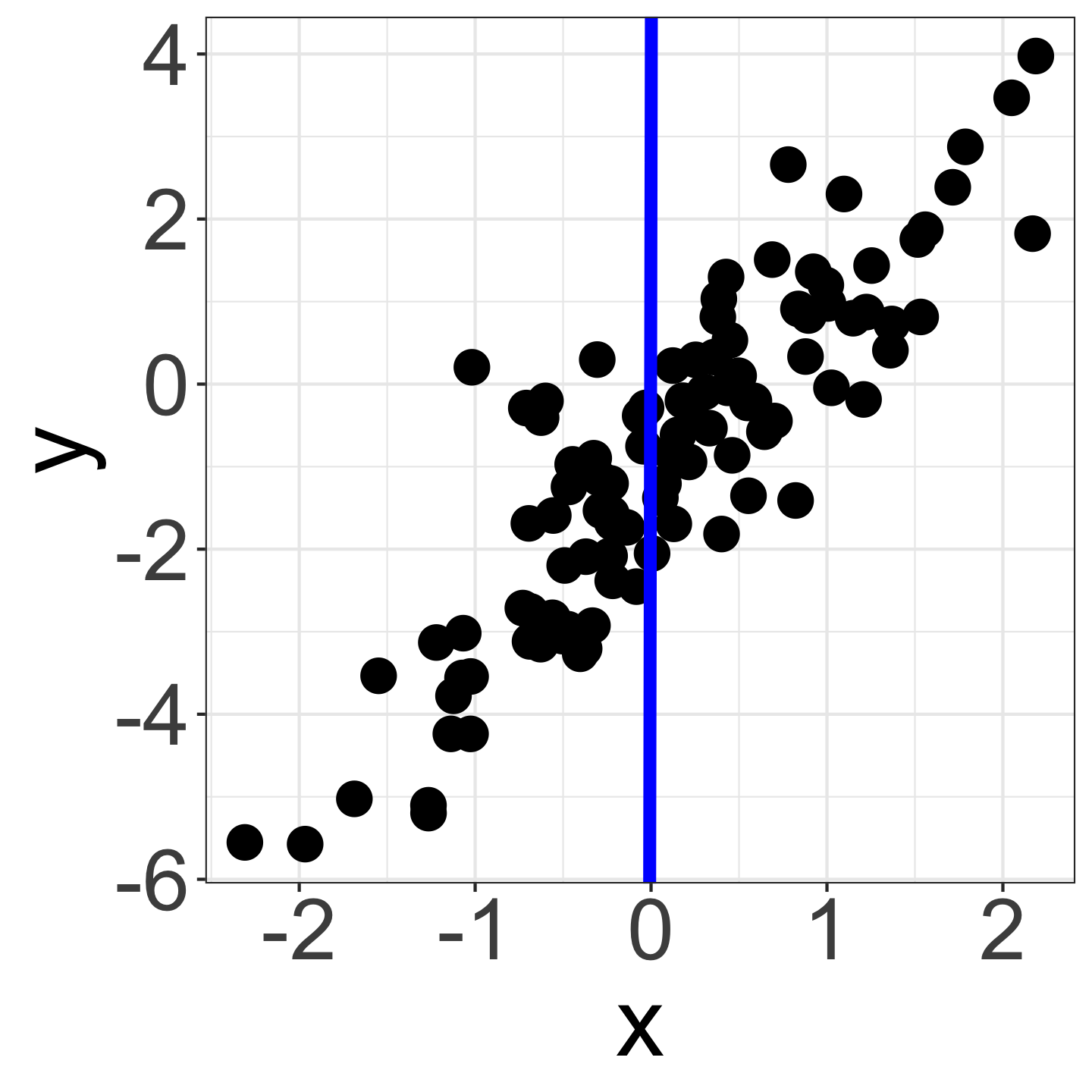
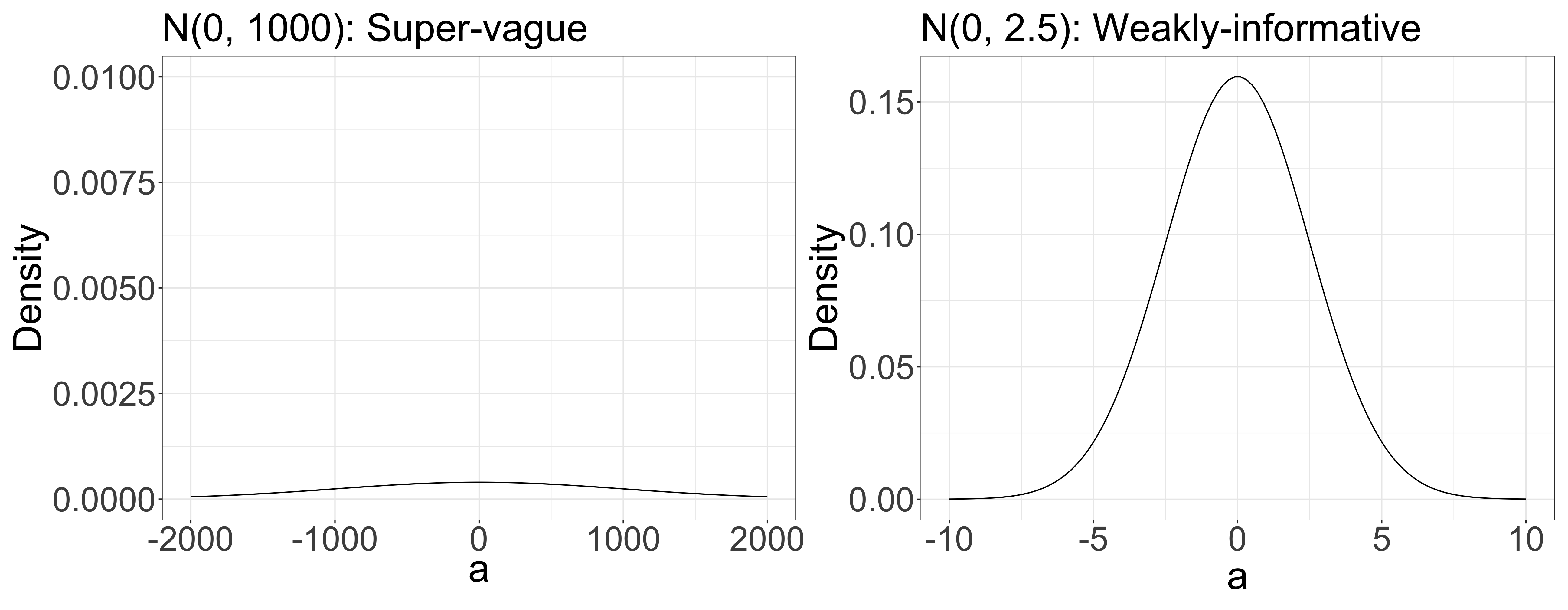
- Considering variables x = {-3, …, 3} and y = {-6, …, 4}. At this point, we don’t know if there is a correlation between x and y.
- However, given the similar scales of x and y, it’s reasonable to guess that a falls within a narrow range (-1000 < a < 1000 or -5 < a < 5 ?).
- For example, y = 100 x + 2 doesn’t work (blue line).
Priors and ecology (simple linear model; y = ax + b)
- Considering variables x = {-3, …, 3} and y = {-6, …, 4}. At this point, we don’t know if there is a correlation between x and y.
- However, given the similar scales of x and y, it’s reasonable to guess that a falls within a narrow range (-1000 < a < 1000 or -5 < a < 5 ?).
Priors and ecology (multilevel model: group-level differences)
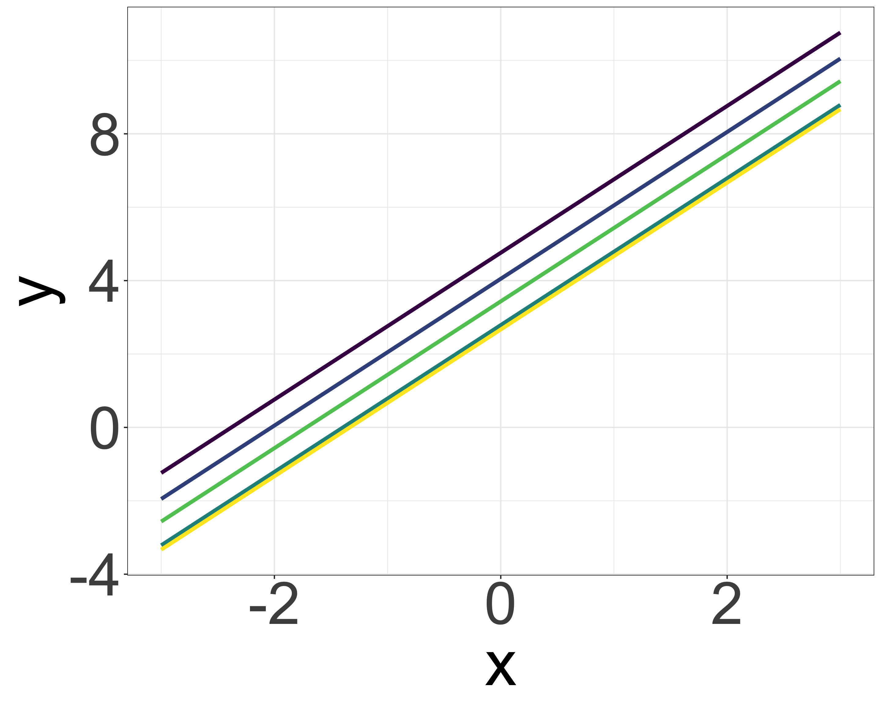
- \(y_i = ax_i + b_j\)
- If the parameter \(b_j\) is similar within each group (e.g., species differences, site differences):
- Likelihood: \(y_i \sim \mathcal{N}(ax_i + b_j, \sigma)\)
- Prior: \(b_j \sim \mathcal{N}(\mu_b, \tau)\)
Priors and ecology (multilevel model: autocorealtion)
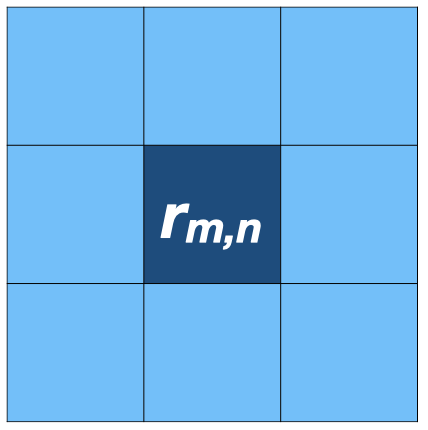
- If the data \(y_i\) is similar to the surrounding samples (e.g., spatial autocorrelation):
- Likelihood: \(y_i \sim \mathcal{N}(\mu + \tilde{r_i}, \sigma)\)
- Prior: \(\tilde{r_i} = r_{m, n} \sim \mathcal{N}(\phi_{m,n}, \tau)\)
- \(\phi_{m,n} = (r_{m-1, n-1} + r_{m, n-1} + r_{m+1, n-1} +\) \(r_{m-1, n} + r_{m+1, n} +\) \(r_{m+1, n-1} + r_{m+1, n} + r_{m+1, n+1})/8\)
Multilevel model
Baseball statistics
https://www.mlb.com/stats/batting-average

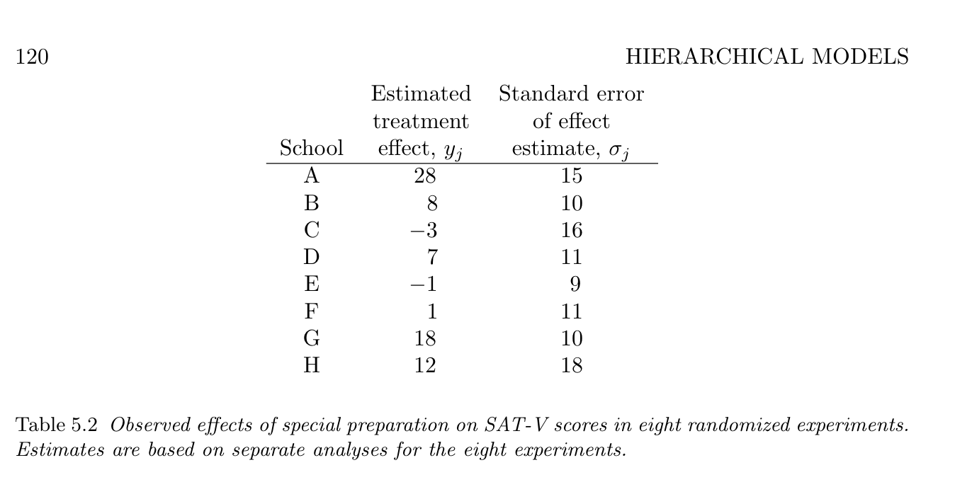
Eight school problem
[1] Rubin, D. B. Estimation in parallel randomized experiments. Journal of Educational Statistics 6, 377–401 (1981).
[2] Gelman, A. et al. Bayesian Data Analysis, Third Edition. (Chapman & Hall/CRC, 2013).
Eight species problem
Newly developed example
What is the survival rate?
Eight species problem (separate estimates)
What is the survival rate?
| sp | n | suv | p_like |
|---|---|---|---|
| A | 41 | 9 | 0.22 |
| B | 45 | 18 | 0.40 |
| C | 32 | 6 | 0.19 |
| D | 18 | 5 | 0.28 |
| E | 33 | 8 | 0.24 |
| F | 26 | 8 | 0.31 |
| G | 46 | 11 | 0.24 |
| H | 16 | 8 | 0.50 |
- If we estimate each species separately, survival rates will be
p_like
Eight species problem (separate estimates)
What is the survival rate?
| sp | n | suv | p_like | p_true |
|---|---|---|---|---|
| A | 41 | 9 | 0.22 | 0.34 |
| B | 45 | 18 | 0.40 | 0.30 |
| C | 32 | 6 | 0.19 | 0.34 |
| D | 18 | 5 | 0.28 | 0.36 |
| E | 33 | 8 | 0.24 | 0.25 |
| F | 26 | 8 | 0.31 | 0.23 |
| G | 46 | 11 | 0.24 | 0.25 |
| H | 16 | 8 | 0.50 | 0.34 |
p_trueranges [0.23, 0.36]p_likeranges [0.19, 0.5]The estimate shows the larger variation
Because of the small sample size (common in ecological studies)
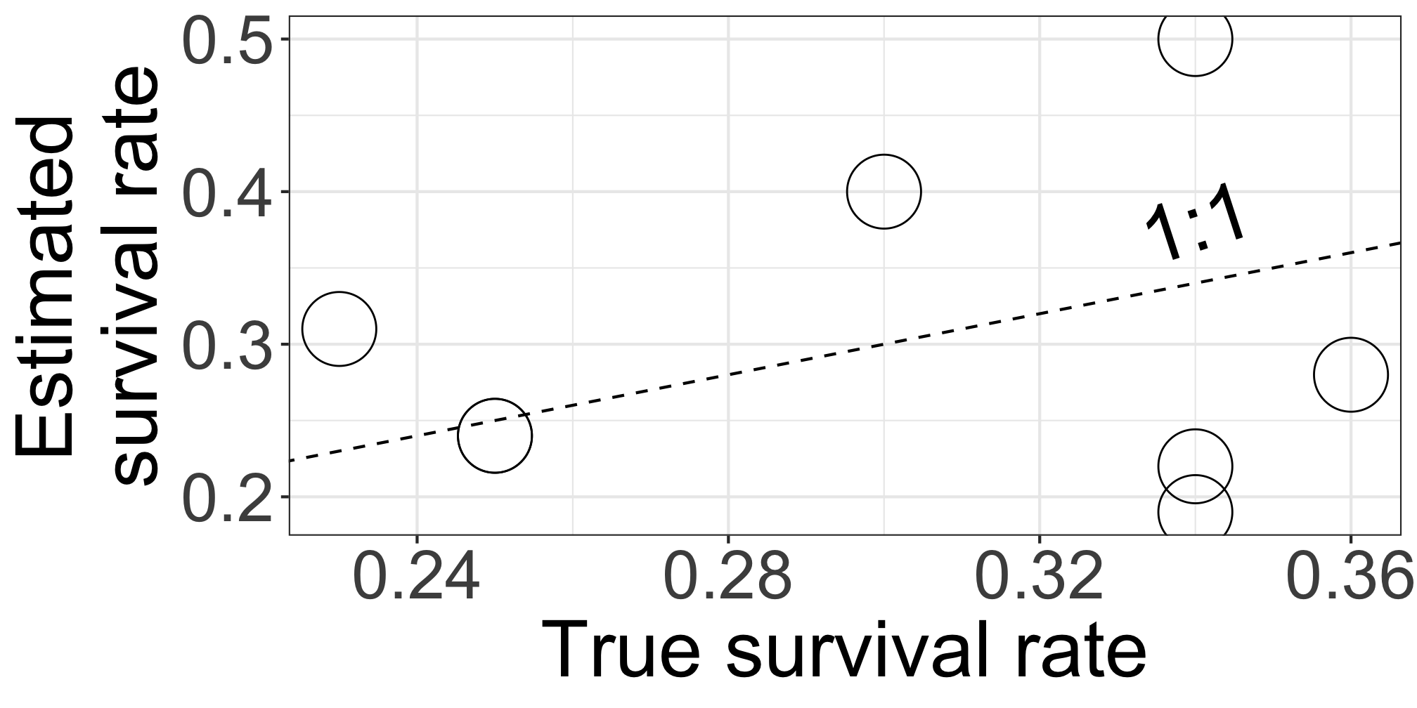
We know p_true because we generated this data using p_true as a known parameter. In practical scenarios, we don’t know p_true.
Two extreme cases (pooled estimates)
- \(S_i \sim \mathcal{B}(N_i, p)\)

- This model doesn’t consider the variation among species
Two extreme cases (separate estimates)
- \(S_i \sim \mathcal{B}(N_i, p_i)\)
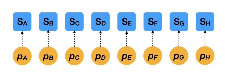
- This model assumes that survival rates are 100% independent among species
More realistic estimates (multilevel models)
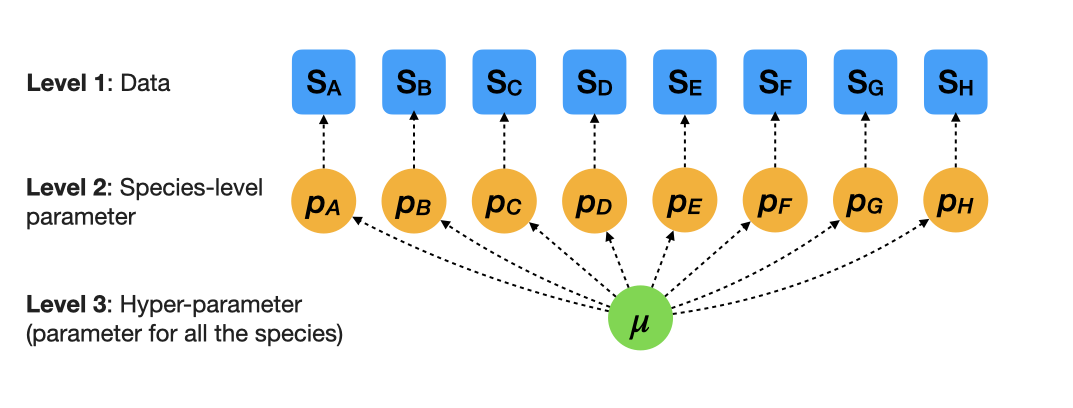
\(S_i \sim \mathcal{B}(N_i, p_i)\)
\(z_i \sim \mathcal{N}(\mu, \sigma)\) where \(z_i = \mathrm{logit}(p_i) = \mathrm{log}\frac{p_i}{1 - p_i}\)
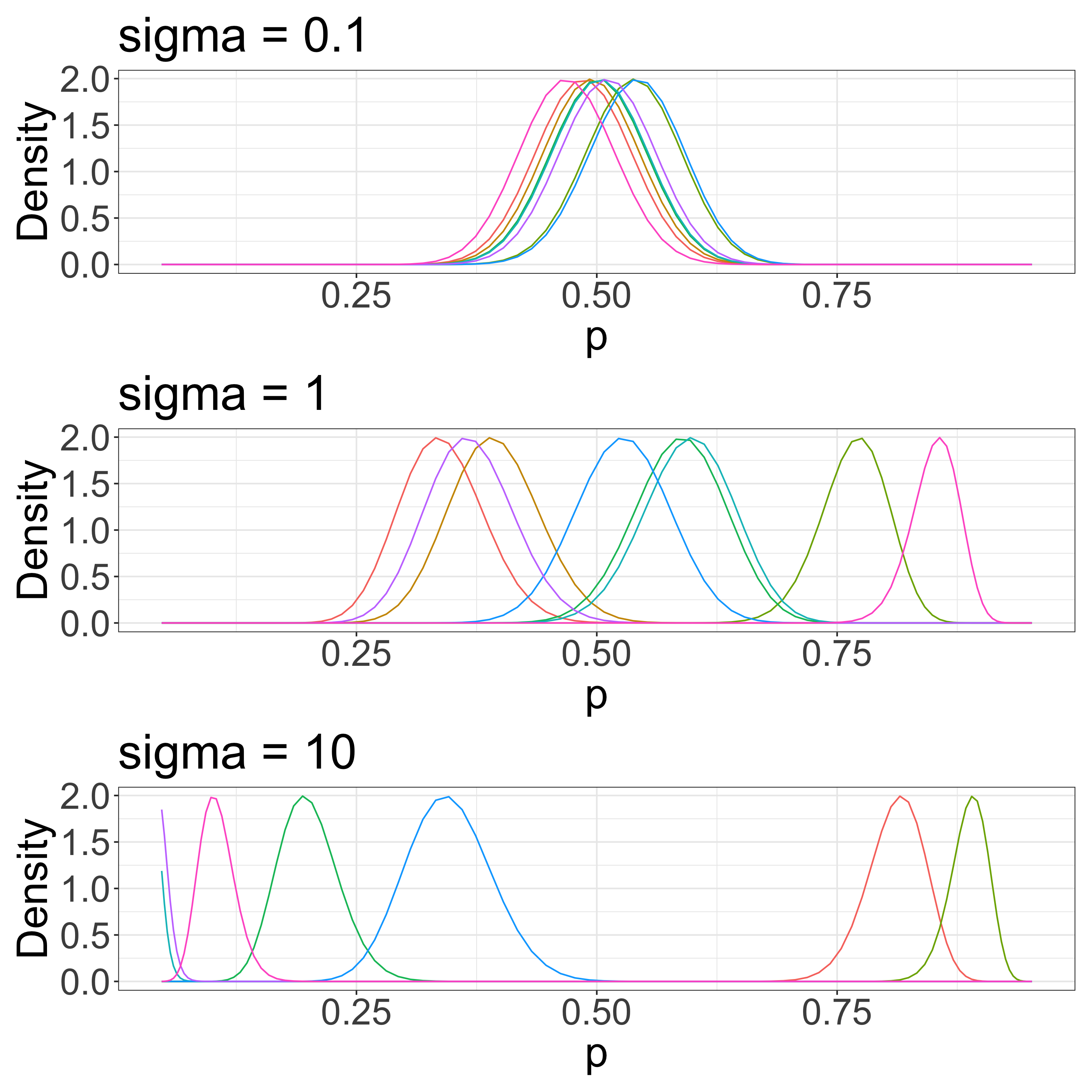
\(\sigma\) determines species variation
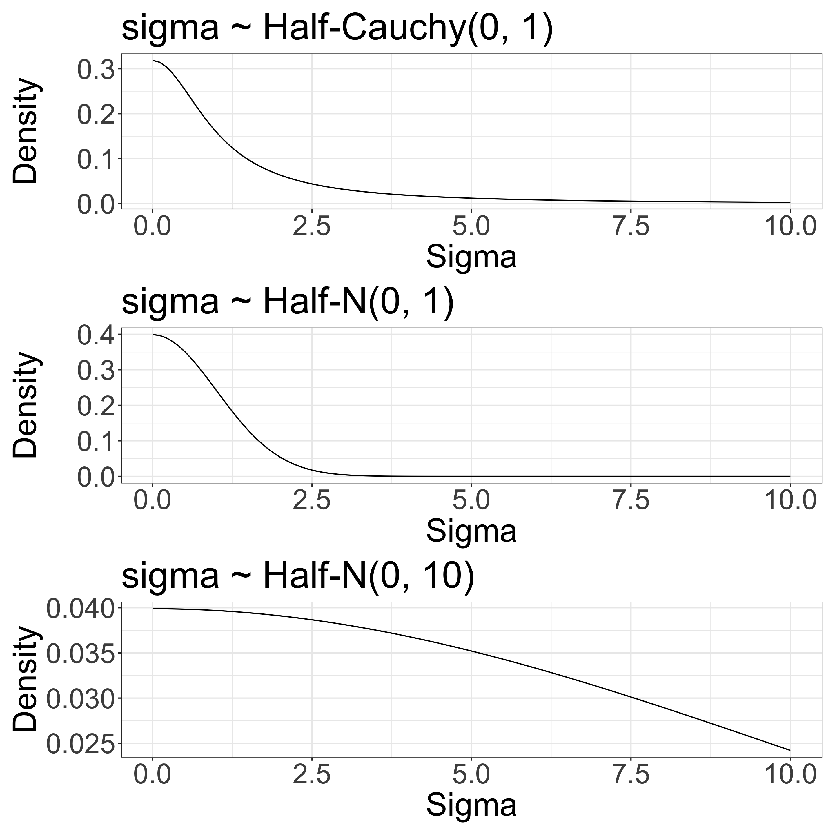
The overall survival rate is 0.5 in this example. We have some sense of a scale for \(\sigma\).
Stan code for a simple multilevel logistic model (non-verbal model)
data {
  int<lower=1> I; // number of species
  array[I] int<lower=0> suv; // number of survivors
  array[I] int<lower=0> N; // number of individuals
  array[I] int<lower=1, upper=I> ii; // integer
}

parameters {
  real mu;
  real<lower=0> sigma;
  vector[I] z_tilde;
}

transformed parameters {
  vector[I] z;
  z = mu + sigma * z_tilde;
}

model {
  mu ~ normal(0, 5);
  z_tilde ~ std_normal();
  sigma ~ std_normal();
  for (i in 1:I)
    suv[i] ~ binomial_logit(N[i], z[ii[i]]);
}

generated quantities {
  vector[I] log_lik;
  vector[I] p = inv_logit(z);
  for (i in 1:I)
    log_lik[i] = binomial_logit_lpmf(suv[i] | N[i], z[ii[i]]);
}
Centered parameterization
\(S_i \sim \mathcal{B}_{logit}(N_i, z_i)\): likelihood
\(z_i \sim \mathcal{N}(\mu, \sigma)\) : prior
\(\sigma \sim \mathcal{N}(0, 1)\): prior
\(\mu \sim \mathcal{N}(0, 5)\): prior
Non-Centered parameterization
\(z_i = \mu + \sigma \cdot \tilde{z_i}\)
\(\tilde{z_i} \sim \mathcal{N}(0, 1)\): prior
Multilevel models yield better estimates
| sp | n | suv | p_like | p_true | p_bayes |
|---|---|---|---|---|---|
| A | 41 | 9 | 0.22 | 0.34 | 0.26 |
| B | 45 | 18 | 0.40 | 0.30 | 0.33 |
| C | 32 | 6 | 0.19 | 0.34 | 0.26 |
| D | 18 | 5 | 0.28 | 0.36 | 0.28 |
| E | 33 | 8 | 0.24 | 0.25 | 0.27 |
| F | 26 | 8 | 0.31 | 0.23 | 0.29 |
| G | 46 | 11 | 0.24 | 0.25 | 0.27 |
| H | 16 | 8 | 0.50 | 0.34 | 0.32 |
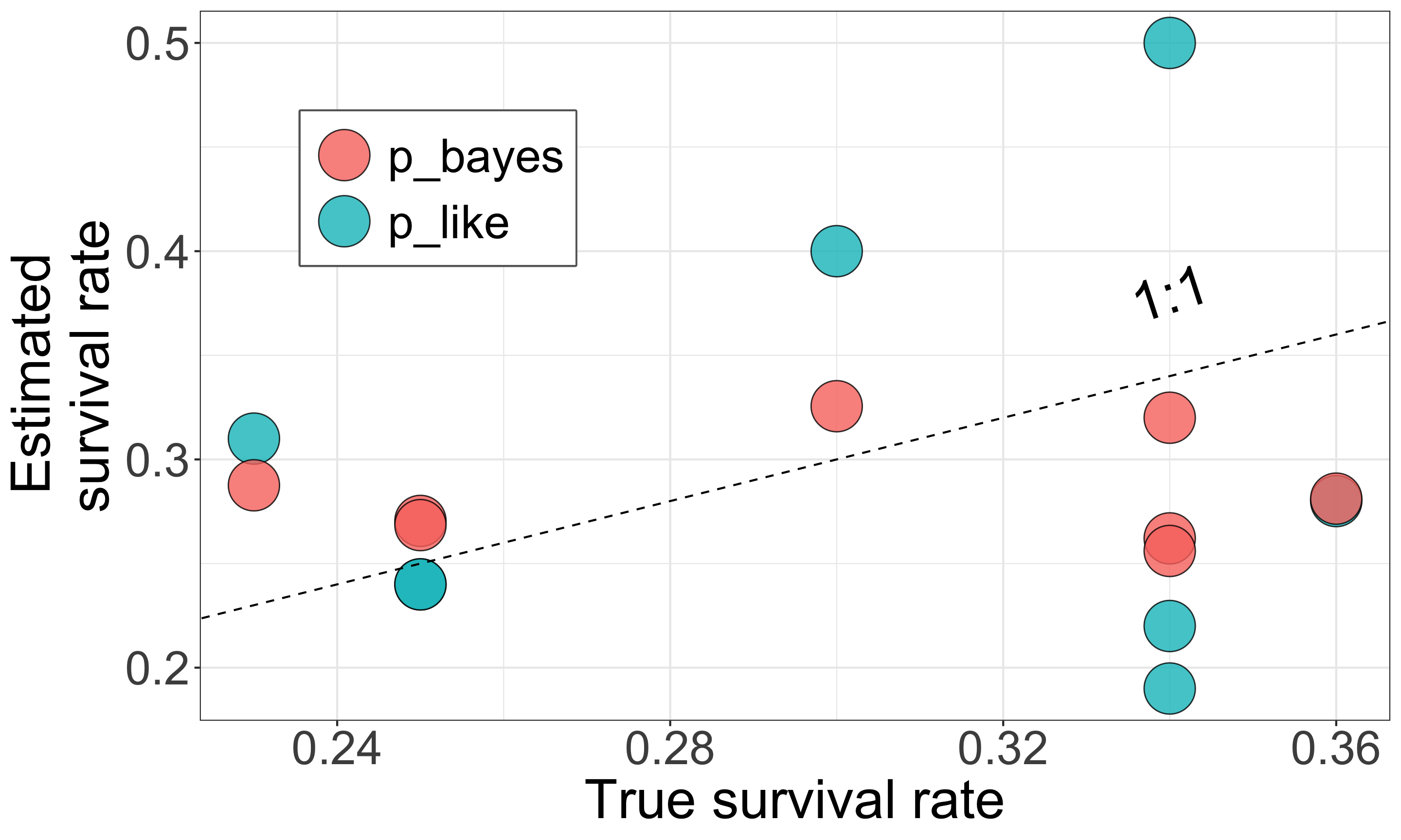
Closed symbols (
p_bayes) align more closely with the 1:1 line, indicating more accurate estimates.This model compensates for limited data by using prior knowledge that species responses are somehow similar and compensates for limited data.
MLE vs. Bayesian estimation
Bayesian estimation (stan)
data {
  int<lower=1> I; // number of species
  array[I] int<lower=0> suv; // number of survivors
  array[I] int<lower=0> N; // number of individuals
  array[I] int<lower=1, upper=I> ii; // integer
}

parameters {
  real mu;
  real<lower=0> sigma;
  vector[I] z_tilde;
}

transformed parameters {
  vector[I] z;
  z = mu + sigma * z_tilde;
}

model {
  mu ~ normal(0, 5);
  z_tilde ~ std_normal();
  sigma ~ std_normal();
  for (i in 1:I)
    suv[i] ~ binomial_logit(N[i], z[ii[i]]);
}

generated quantities {
  vector[I] log_lik;
  vector[I] p = inv_logit(z);
  for (i in 1:I)
    log_lik[i] = binomial_logit_lpmf(suv[i] | N[i], z[ii[i]]);
}
MLE vs. Bayesian estimation
Bayesian estimation (brms)
- Several packages, like
brmsandrstanarm, offer Bayesian estimation using syntax similar tolme4.
MLE vs. Bayesian estimation
MLE (e.g., lme4)
\(L(\mu, \sigma) = \prod_i \int_{-\infty}^{\infty} \mathcal{B}(S_i \mid N_i, p_i) \times \mathcal{N}(\mathrm{logit}(p_i) \mid \mu, \sigma) dp_i\)
Analytically find \(\mu\) and \(\sigma\) to maximize \(L\)
An analytical solution is often not available (this example is easy though)
Bayesian estimation
\(P(\mu, \sigma \mid S_i, N_i) \propto \prod_i \mathcal{B}(S_i \mid N_i, p_i) \times \prod_i \mathcal{N}(\mathrm{logit}(p_i) \mid \mu, \sigma) \times\) \(\;\;\;\;\;\;\;\;\;\;\;\;\;\;\;\;\;\;\;\;\;\;\;\;\;\mathcal{N}(\mu \mid 0, 5) \times \mathcal{N}(\sigma \mid 0, 2.5)\)
Numerically find \(\mu\) and \(\sigma\) to maximize \(P\) (aka MCMC)
MCMC works even if an analytical solution is not available
Bayes’s theorem supports the use of MCMC
Summary
Why Bayesian estimation is useful
We can use a priori information about parameters in our model
Models are flexible
MCMC works even if models are complicated
Why multilevel models are important
Multilevel models have a good balance between pooled estimates and separate estimates, which is useful for practical sample sizes
Multilevel models handle nested or hierarchical data structures, a common and important scenario in ecological research (e.g., trees within species, community within sites, etc.).
References
Gelman, A. et al. Bayesian Data Analysis, Third Edition. (Chapman & Hall/CRC, 2013)
AIcia Solid Project (in Japanese and Math)
