Bayesian estimation for ecology

🧑🏻‍💻 Masatoshi Katabuchi @ XTBG, CAS

• mattocci27@gmail.com
• @mattocci
• github.com/mattocci27/bayes-afec
• https://mattocci27.github.io

November 3, 2025 Experimental Design and Statistics in R, AFEC, XTBG

hoge

Objectives

• We Learn

  • Why Bayesian estimation is useful

  • Why multilevel models are important

  • How to use and code Bayesian models in Stan and R

• coding exercises are not the focus of this workshop
• it will take a couple of days
• idea of Bayesian in ecology

Outline: From Likelihood to Hierarchical Bayesian Models in Ecology

Bayesian Foundations

• Likelihood

• Multilevel Models (Conceptual Motivation)

• Conditional Probability and Bayes’ Theorem

• Prior

• Multilevel Model Revisited

Modeling with Stan

• Tools for Bayesian Modeling

• Stan Coding Session (separate HTML material)

Likelihood

Assuming everyone knows the concept of likelihood

correct?

Likelihood and probability density distribution (Normal)

\(f(x \mid \mu, \sigma) = \frac{1}{\sqrt{2\pi\sigma^2}}\mathrm{exp} \bigl[{-\frac{1}{2}\bigl\{\frac{x-\mu}{\sigma}}\bigr\}^2\bigr]\)

• P(data | parameters): Probability of observing the data given the parameters.

• e.g., when your model is \(x_i \sim \mathcal{N}(\mu = 0, \sigma^2 = 1)\) (normal distribution with mean 0 and variance 1), what is the probability density at x = 1.96?

1 / sqrt(2 * pi * 1) * exp(-1/2 * (1.96 - 0)^2 / 1)

  [1] 0.05844094

• \(P(x = 1.96 \mid \mu = 0, \sigma = 1)\)

dnorm(1.96, mean = 0, sd = 1)

  [1] 0.05844094

• likelihood is all about probability density (mass) function (normal, log-normal, poisson, beta, gamma, binomial, negative-binomial…)

Likelihood and probability mass distribution (Poisson)

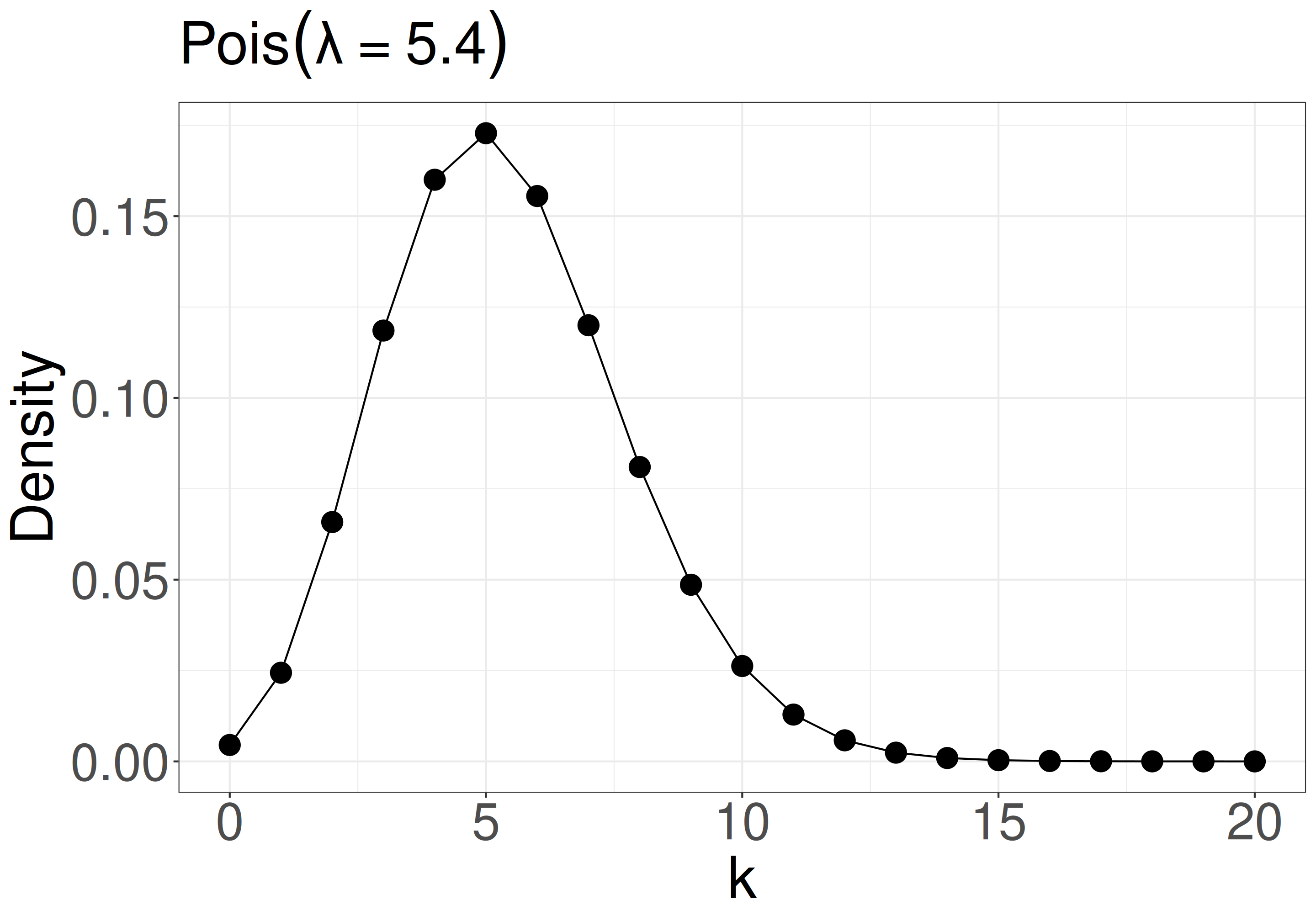
\(f(k \mid \lambda) = \frac{\lambda^k e^{-\lambda}}{k!}\)

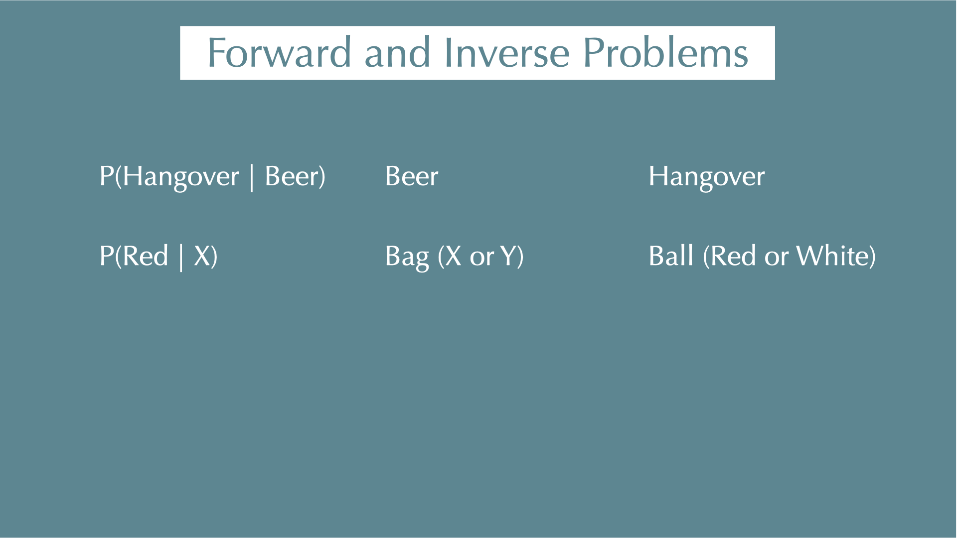
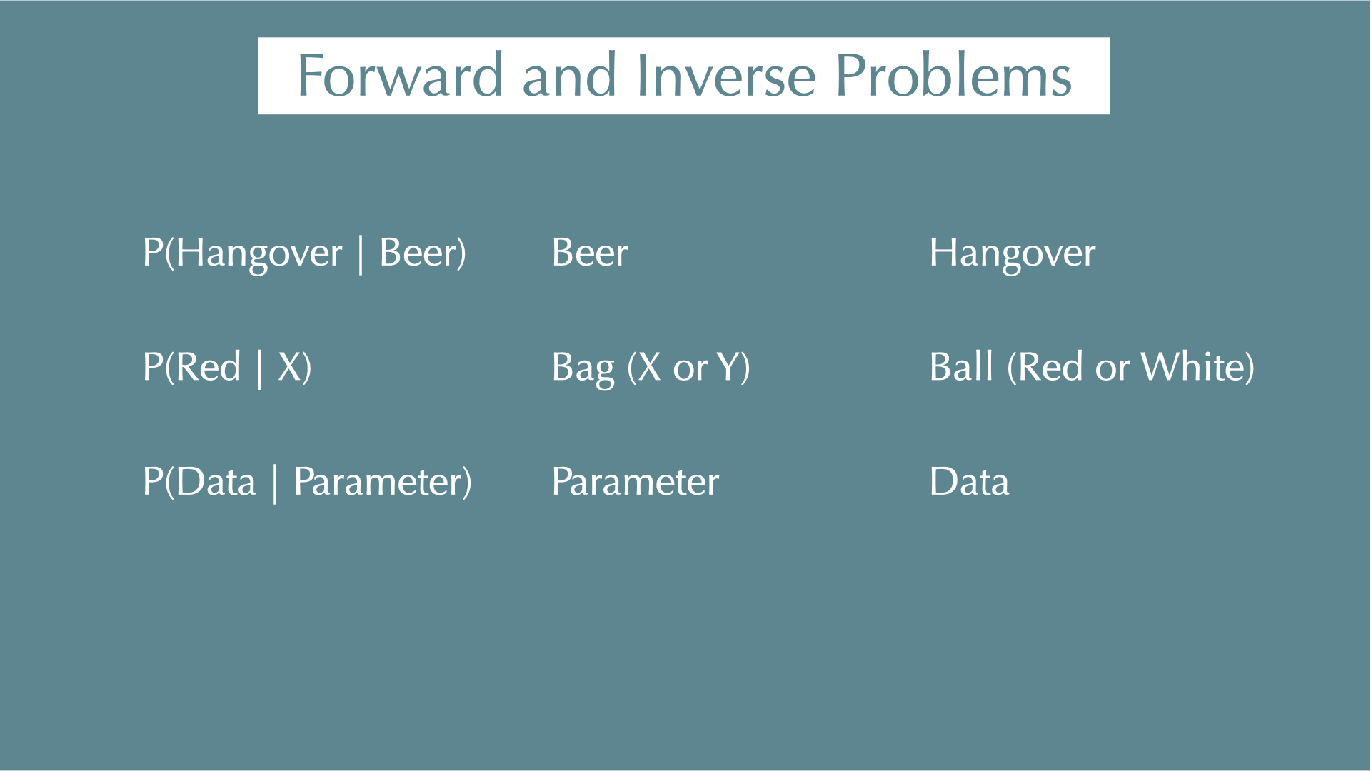
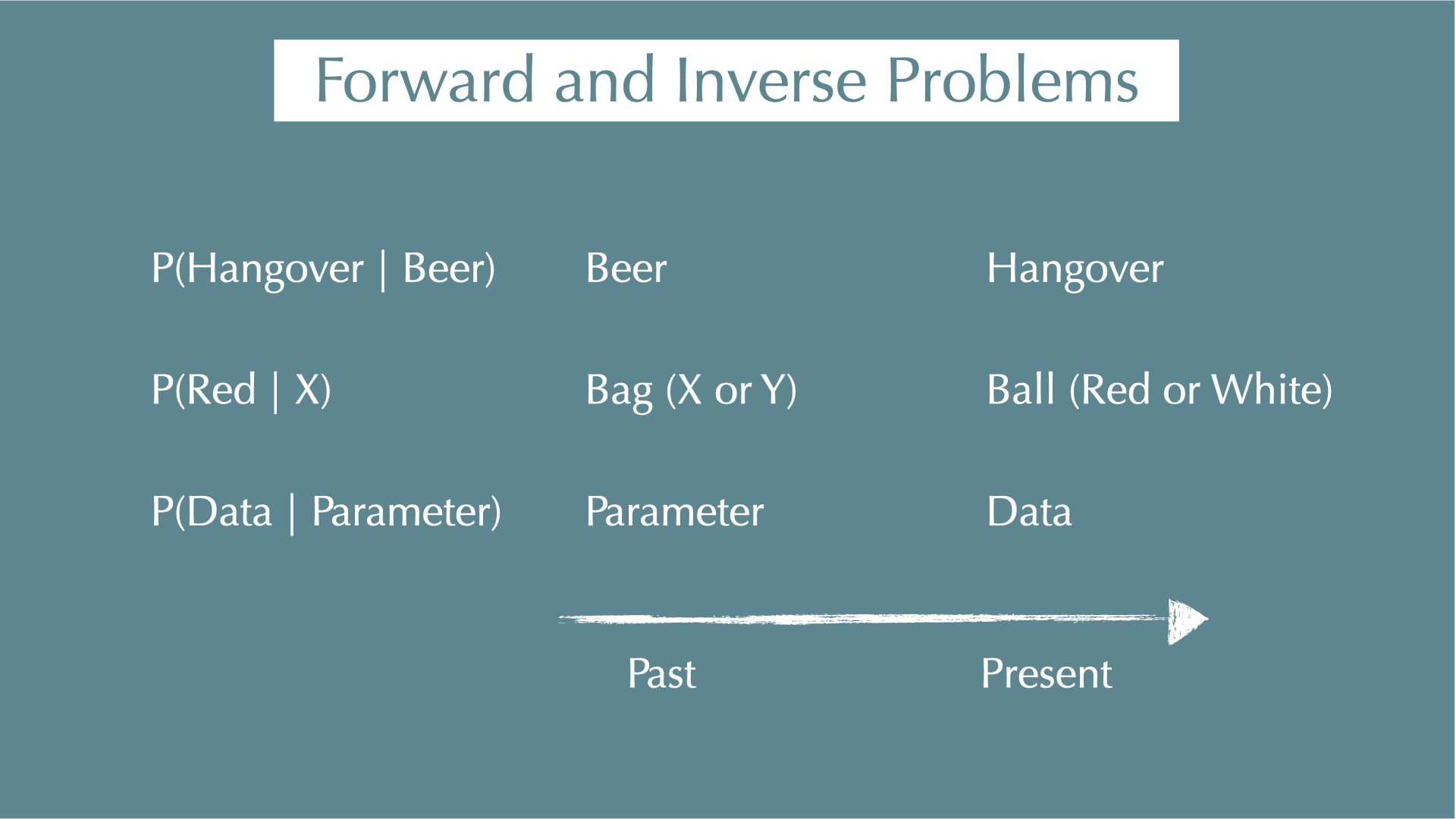
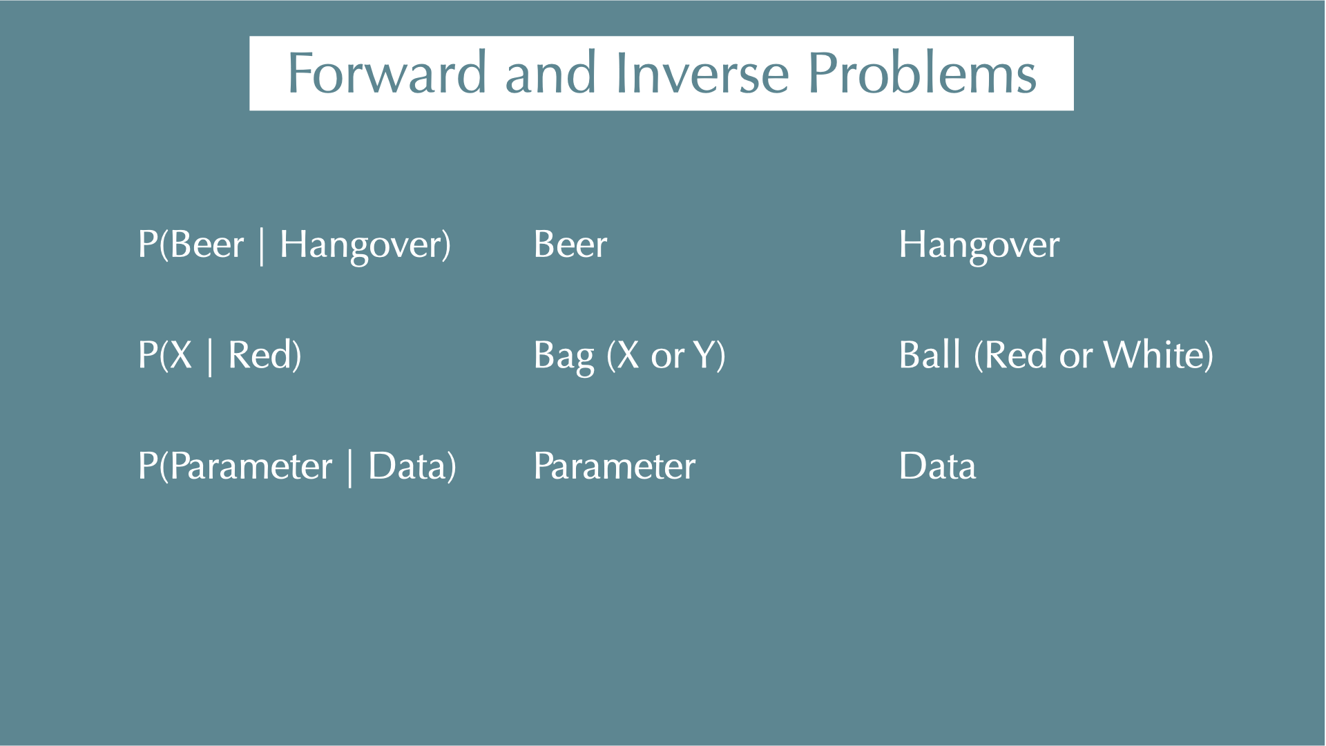
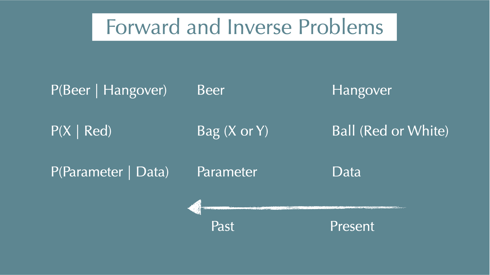
• P(data | parameters): Probability of observing the data given the parameters.

• e.g., when your model is \(k_i \sim \mathcal{Pois}(\lambda = 5.4)\) (Poisson distribution with mean and variance = 5.4), what is the probability mass at k = 8?

(5.4^8 * exp(-5.4)) / factorial(8)

  [1] 0.08099148

• \(P(k = 8 \mid \lambda = 5.4)\)

dpois(8, lambda = 5.4)

  [1] 0.08099148

• likelihood is all about probability density (mass) function (normal, log-normal, poisson, beta, gamma, binomial, negative-binomial…)

Likelihood (Back to Normal distribution)

When your data is x = {-1.5, 0, 1.5} and your model is \(x \sim \mathcal{N}(0, 1)\), what is the probability of observing x?

• \(L = P(-1.5 \mid 0, 1) \times P(0 \mid 0, 1) \times P(1.5 \mid 0, 1)\)
• \(\mathrm{ln}\;L = \mathrm{ln}\;P(-1.5 \mid 0, 1) + \mathrm{ln}\;P(0 \mid 0, 1) + \mathrm{ln}\;P(1.5 \mid 0, 1)\)

dnorm(-1.5, mean = 0, sd = 1, log = TRUE) + dnorm(0, mean = 0, sd = 1, log = TRUE) + dnorm(1.5, mean = 0, sd = 1, log = TRUE)

  [1] -5.006816

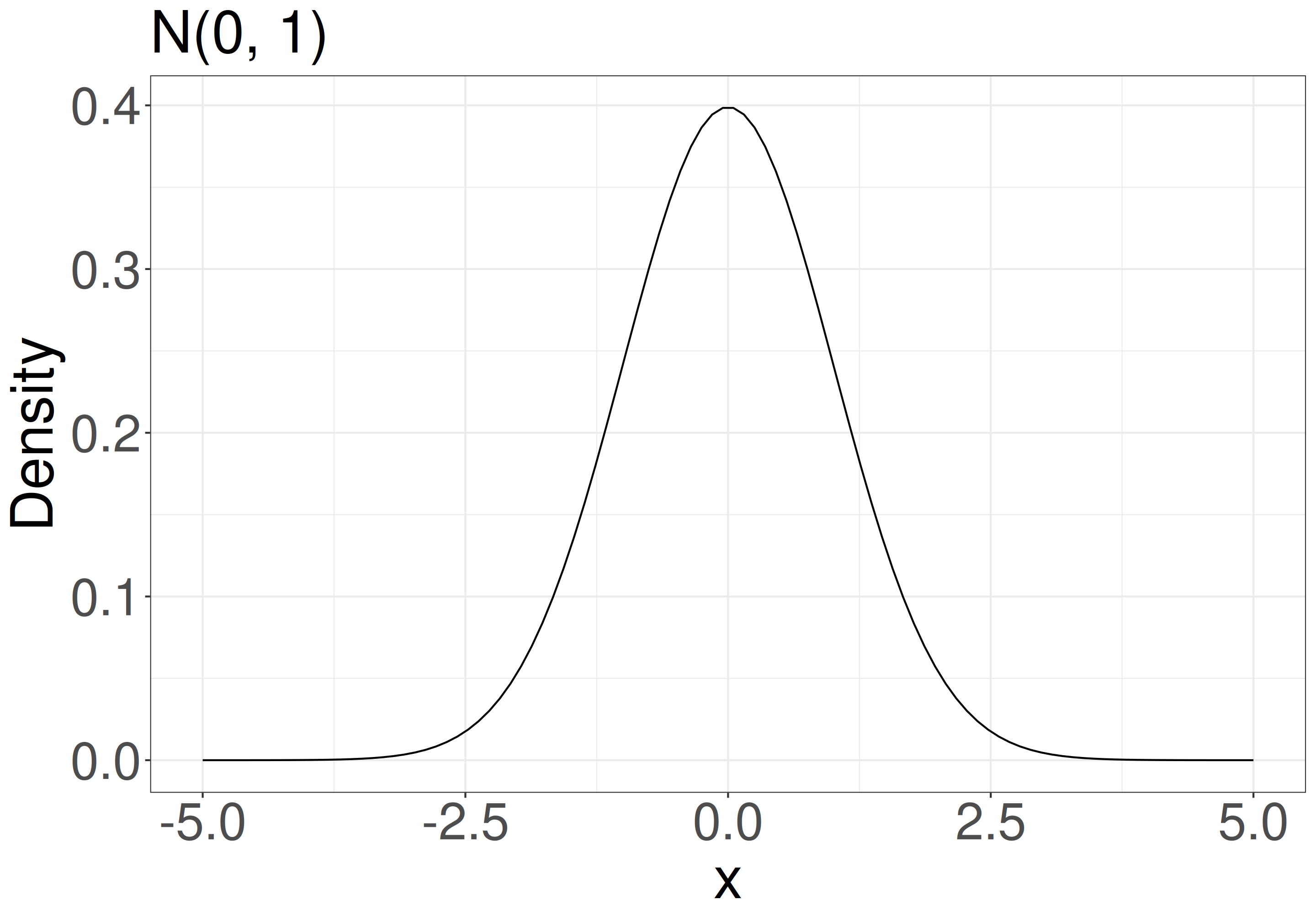
Likelihood

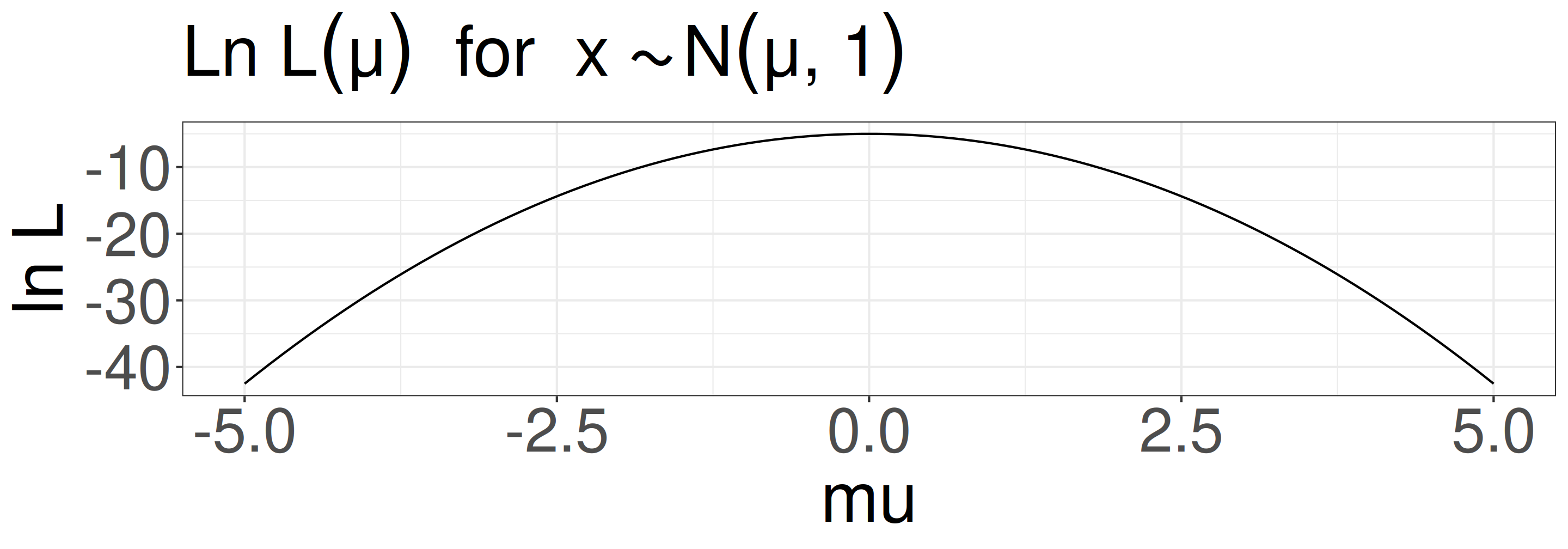
• Because we usually don’t know the true parameters (\(\mu\) and \(\sigma\)), we need to find the parameters that maximize the likelihood function (MLE: Maximum Likelihood Estimation).

  • e.g., for a linear model \(y_i = ax_i + b\), we usually assume that \(y_i \sim \mathcal{N}(\mu_i = ax_i + b, \sigma^2)\), and we want to find the parameters \(a\), \(b\), and \(\sigma\) that maximize the likelihood function: \(P(y_i \mid ax_i + b, \sigma)\)

  • In the previous example, \(\mu\) = 0 makes the likelihood maximum.

Maximum Likelihood Estimation (MLE)

• 2 survivors out of 5 seedlings: What is the survival probability of seedlings?

• \(p\): survival rates, \(1-p\): mortality rate

• \(L = {}_5C_2 p^2(1-p)^3\) (Binomial distribution)

• \(\mathrm{ln}\;L = \mathrm{ln}\;{}_5C_2 + 2\mathrm{ln}\;p + 3\mathrm{ln}(1-p)\)

• \(\frac{d}{dp}\mathrm{ln}\;L = \frac{2}{p} - \frac{3}{1-p} = 0\)

• Solve: \(p = \frac{2}{5}\)

Multilevel Models (Conceptual Motivation)

Negative density dependence (NDD)

“…rare species suffered more from the presence of conspecific neighbors than common species did, suggesting that conspecific density dependence shapes species abundances in diverse communities.”

- Comita et al. 2010 -

NDD can maintain diversity in communities by preventing common species from dominating the community.

Multilevel model (verbal model: NDD example)

H: Rare species tend to be rare because they suffer stronger conspecific NDD than common species.

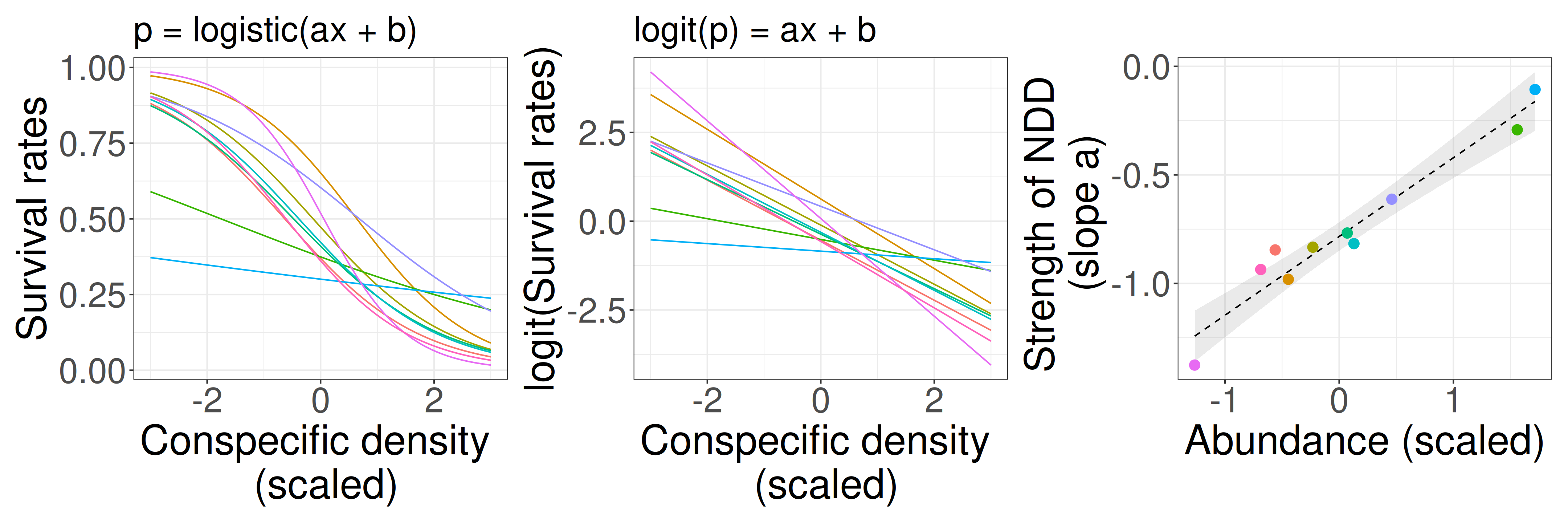
There is negative density dependence (NDD) of seedling survival rate, and the strength of NDD varies among species. The strength of NDD depends on species abundance.

• Survival rates p ~ conspecific density x (individual-level, logistic regression).

• Slopes a ~ species abundance (species-level).

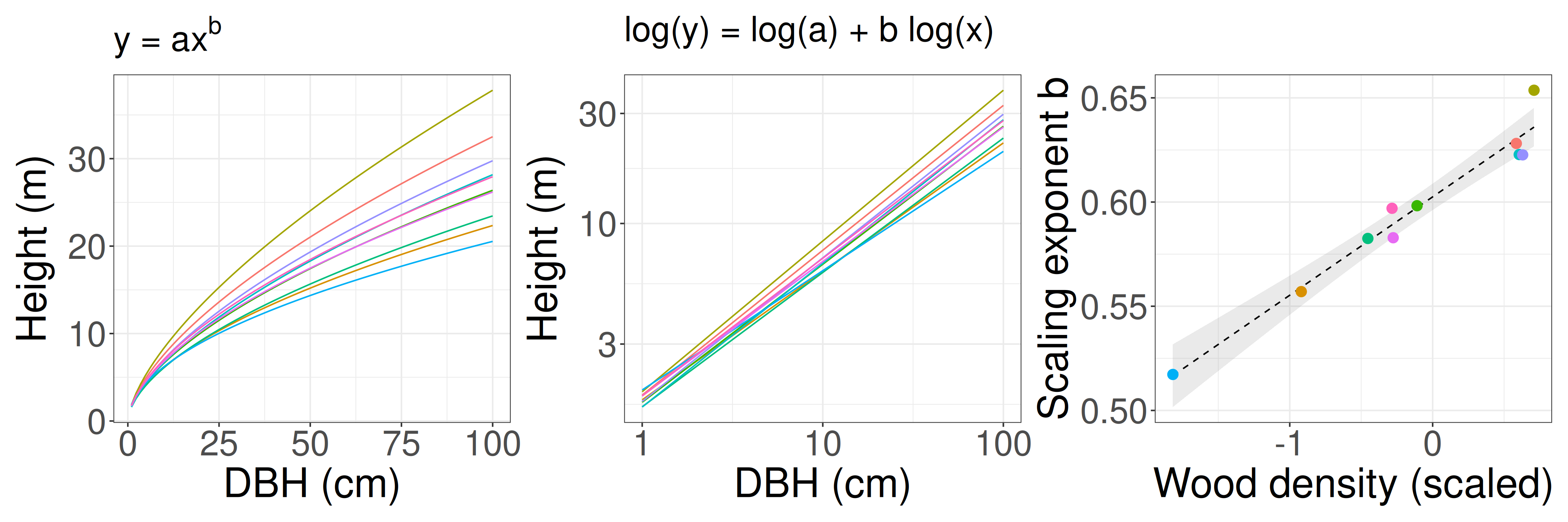
Multilevel model (verbal model: tree allometry example)

H: Dense wood can support taller trees than less dense wood.

There is a power-law relationship (\(y =ax^b\)) between tree diameter (DBH) and tree maximum height, and the power-law exponent varies among species. Those relationships depend on wood density.

• Tree height y ~ DBH x (individual-level)

• Slope b ~ wood density (species-level)

Code implementation: two-stage MLE

Individual-level model: GLMM

fit_ind <- lme4::glmer(
  cbind(suv, n - suv) ~  cons + (1 + cons | sp),
  data = dummy, family = binomial)

• (1 + cons | sp) — random intercept and slope across species.

• We need to extract the slope coefficients for each species from fit_ind and make new_data.

Group-level model: LM

fit_gr <- lm(slope_coef ~  abund, data = new_data)

• This method has low statistical power.

Code implementation: Simultaneous MLE approach

fit_mle <- lme4::glmer(
  cbind(suv, n - suv) ~  cons + abund + cons:abund + (1 + cons | sp),
  data = dummy, family = binomial)

• cons:abund — species-level predictor (abundance) modifying NDD strength.
• (1 + cons | sp) — random intercept and slope across species.
• Combines both levels into a single model.
• Often work for simple models and data.

Code implementation: Bayesian GLMM with brms

fit_bayes <- brms::brms(
  cbind(suv, n - suv) ~  cons + abund + cons:abund + (1 + cons | sp),
  data = dummy, family = binomial())

• Syntax is similar to lme4::glmer().
• Works well for most cases.

Looking ahead: full Bayesian implementation in Stan

data{
  int<lower=1> N; // number of samples
  int<lower=1> J; // number of sp
  int<lower=1> K; // number of tree-level preditors (i.e, CONS, HETS,...)
  int<lower=1> L; // number of sp-level predictors (i.e., interecept, SLA,...)
  matrix[N, K] x; // tree-level predictor
  matrix[L, J] u; // sp-level predictor
  array[N] int<lower=0, upper=1> suv; // 1 or 0
  array[N] int<lower=1, upper=J> sp; // integer
}

parameters{
  matrix[K, L] gamma;
  matrix[K, J] z;
  cholesky_factor_corr[K] L_Omega;
  vector<lower=0, upper=pi() / 2>[K] tau_unif;
}

transformed parameters{
  matrix[K, J] beta;
  vector<lower=0>[K] tau;
  for (k in 1:K) tau[k] = 2.5 * tan(tau_unif[k]);
  beta = gamma * u + diag_pre_multiply(tau, L_Omega) * z;
}

model {
  vector[N] mu;
  to_vector(z) ~ std_normal();
  L_Omega ~ lkj_corr_cholesky(2);
  to_vector(gamma) ~ normal(0, 2.5);
  for (n in 1:N) {
    mu[n] = x[n, ] * beta[, sp[n]];
  }
  suv ~ bernoulli_logit(mu);
}

generated quantities {
  vector[N] log_lik;
  corr_matrix[K] Omega;
  Omega = multiply_lower_tri_self_transpose(L_Omega);
  for (n in 1:N) {
    log_lik[n] = bernoulli_logit_lpmf(suv[n] | x[n, ] * beta[, sp[n]] +
      phi[plot[n]] + xi[census[n]] + psi[tag[n]]);
  }
}

• \(s_{i,j} \sim \mathcal{B}(p_{i, j})\): likelihood

• \(\mathrm{logit}(p_{i,j}) = \boldsymbol{x_{i}} \cdot \boldsymbol{\beta_{j}}\): individual-level model

• \(\boldsymbol{\beta_j} = \boldsymbol{\gamma_k} \cdot \boldsymbol{u_j} + \mathrm{diag}(\boldsymbol{\sigma})\cdot \boldsymbol{L} \cdot \boldsymbol{z}\): species-level model

• \(L \sim \mathrm{LkjCholesky}(\eta)\): prior (?)

• \(z_j \sim \mathcal{N}(0, 1)\): prior (?)

• \(\tau \sim \mathrm{Cauchy}(0, 2.5)\): prior (?)

• \(\gamma_k \sim \mathcal{N}(0, 2.5)\): prior (?)

I won’t explain this now — but this is the kind of model we’ll build after learning Bayes’s theorem, priors, and a bit of linear algebra.

Conditional Probability and Bayes’ Theorem

Conditional Probability and Bayes’ Theorem

\[ P(A \mid B) = \frac{P(B \mid A) \times P(A)}{P(B)} \]

• Conditional probability

• Bayes’ Theorem

• Forward / inverse problems

• Revisiting Bayes

Probability

Probility of A:

\[ P(A) = \frac{A}{U} \]

e.g., probability of rolling a dice and getting an odd number is 3/6 = 1/2

Conditional Probability

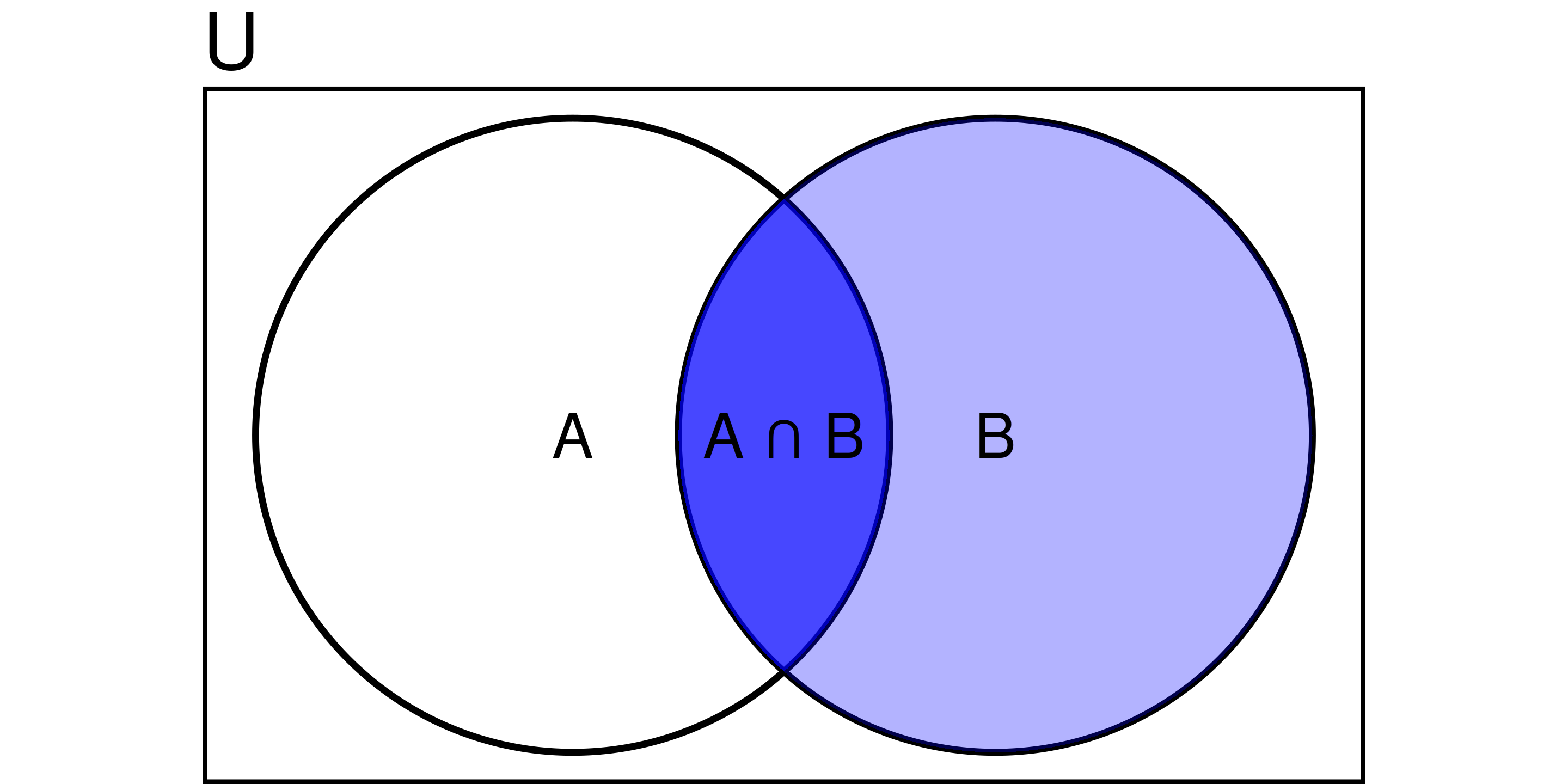
Probability of A occurring given B has already occurred:

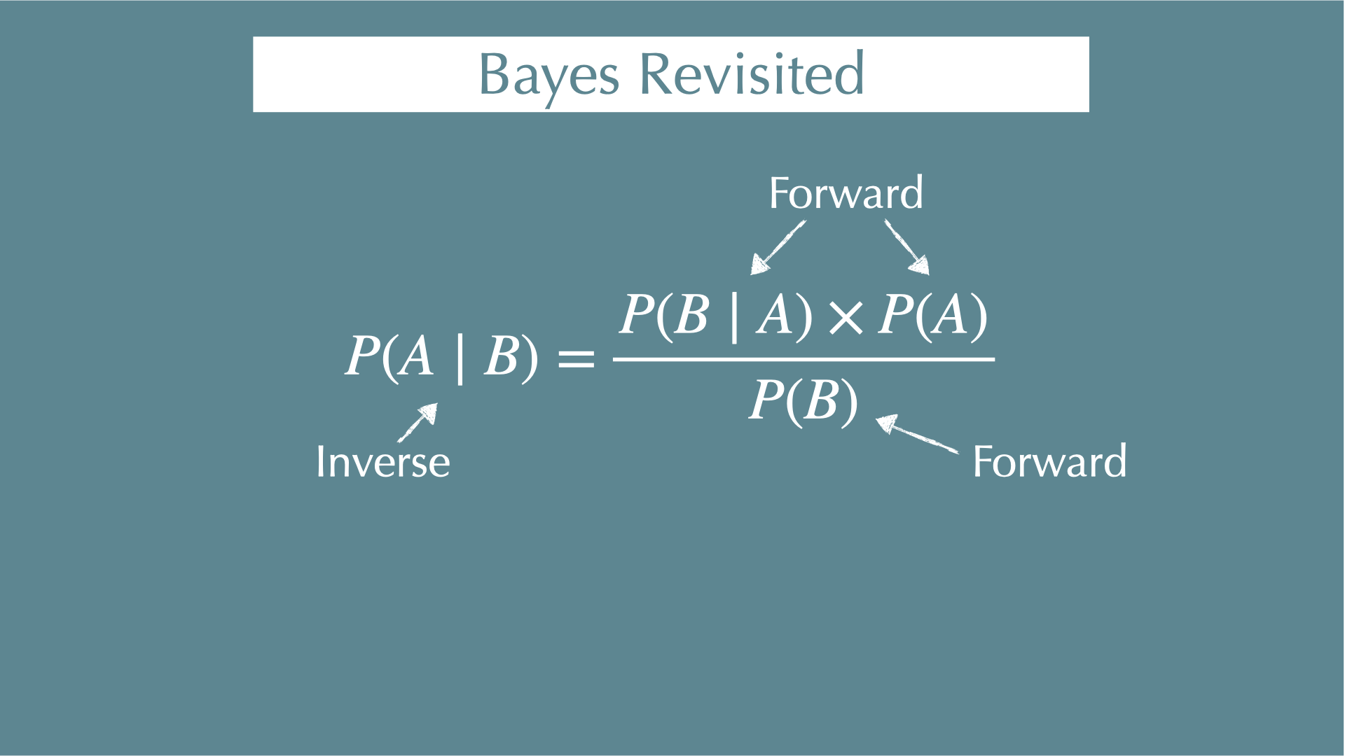
\[ P(A \mid B) = \frac{P(A \cap B)}{P(B)} \]

e.g.,

• P(hangover) = 4%
• P(baiju) = 1.5%
• P(hangover | baiju) = 85%.

• probability A occurs given B
• vertical bar = given
• at least 1 day for each month
• the next day after I had beer
• the next day after I had baiju

Bayes’ Theorem

\[ P(B \mid A) = \frac{P(A \cap B)}{P(A)} \]

\[ P(A \mid B) = \frac{P(A \cap B)}{P(B)} \]

\[ P(A \mid B) \times P(B) = P(B \mid A) \times P(A) \]

\[ P(A \mid B) = \frac{P(B \mid A) \times P(A)}{P(B)} \]

Why is this useful?

Forward and Inverse Problems: PCR and disease example

➡️Forward problem: If you are infected, what is the probability that PCR test is positive?

\(P(\text{Positive} \mid \text{Infected})\): 95%

This is what the lab test is designed to estimate — how likely we are to observe a positive signal given the known infection status (e.g., 95 out of 100 infected samples test positive).

Forward and Inverse Problems: PCR and disease example

🔁Inverse problem (Bayesian): If the PCR test is positive, what is the probability that you are infected?

• \(P(\text{Infected} \mid \text{Positive}) = \frac{P(\text{Positive} \mid \text{Infected}) \cdot P(\text{Infected})}{P(\text{Positive})} \approx 2.4\%\)

This isn’t intuitive, but it’s the probability we actually care about — how likely someone is to be infected, given a positive test result.

Bayes’ theorem

\[ \textcolor{#d95f02}{ P(\mathrm{Parameter} \mid \mathrm{Data}) } = \frac{ \textcolor{#1b9e77} { P(\mathrm{Data} \mid \mathrm{Parameter}) } \times \textcolor{#7570b3} { P(\mathrm{Parameter})} } {P(\mathrm{Data})} \]

• \(\textcolor{#d95f02}{P(\mathrm{Parameter} \mid \mathrm{Data})}\)

  • What we want to estimate (posterior): When we got our data, what were the parameters behind the data (e.g., coefficients of regressions)?

• \(\textcolor{#1b9e77}{P(\mathrm{Data} \mid \mathrm{Parameter})}\)

  • When we know our parameters, what is the probability of getting our data? (i.e., likelihood)

• \(\textcolor{#7570b3}{P(\mathrm{Parameter})}\)

  • Probability to get our parameters. This is what we assume for our parameter before we see any data (i.e., prior?? — next section).

• \(P(\mathrm{Data})\)

  • Independent with parameters (i.e., constant)

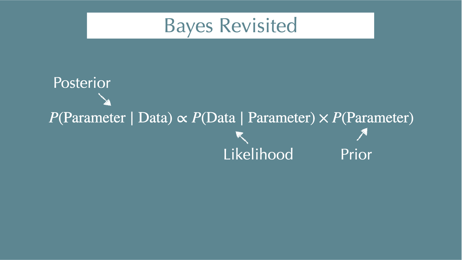
Prior

Prior vs. Data: MLE and Bayesian comparison (Coin Toss)

We compare two coins, A and B, with the same prior but different likelihood (due to data sizes) to illustrate how prior beliefs influence posterior estimates.

MLE

• A: 2 head out of 3 tosses -> P(H) = 2/3 = 0.666
• B: 60 heads out of 100 tosses -> P(H) = 60/100 = 0.6

Bayesian

• \(\textcolor{#1b9e77}{L_A = {}_3C_2 p^2 (1-p)^1}\)

• \(\textcolor{#1b9e77}{L_B = {}_{100}C_{60} p^{60} (1-p)^{40}}\)

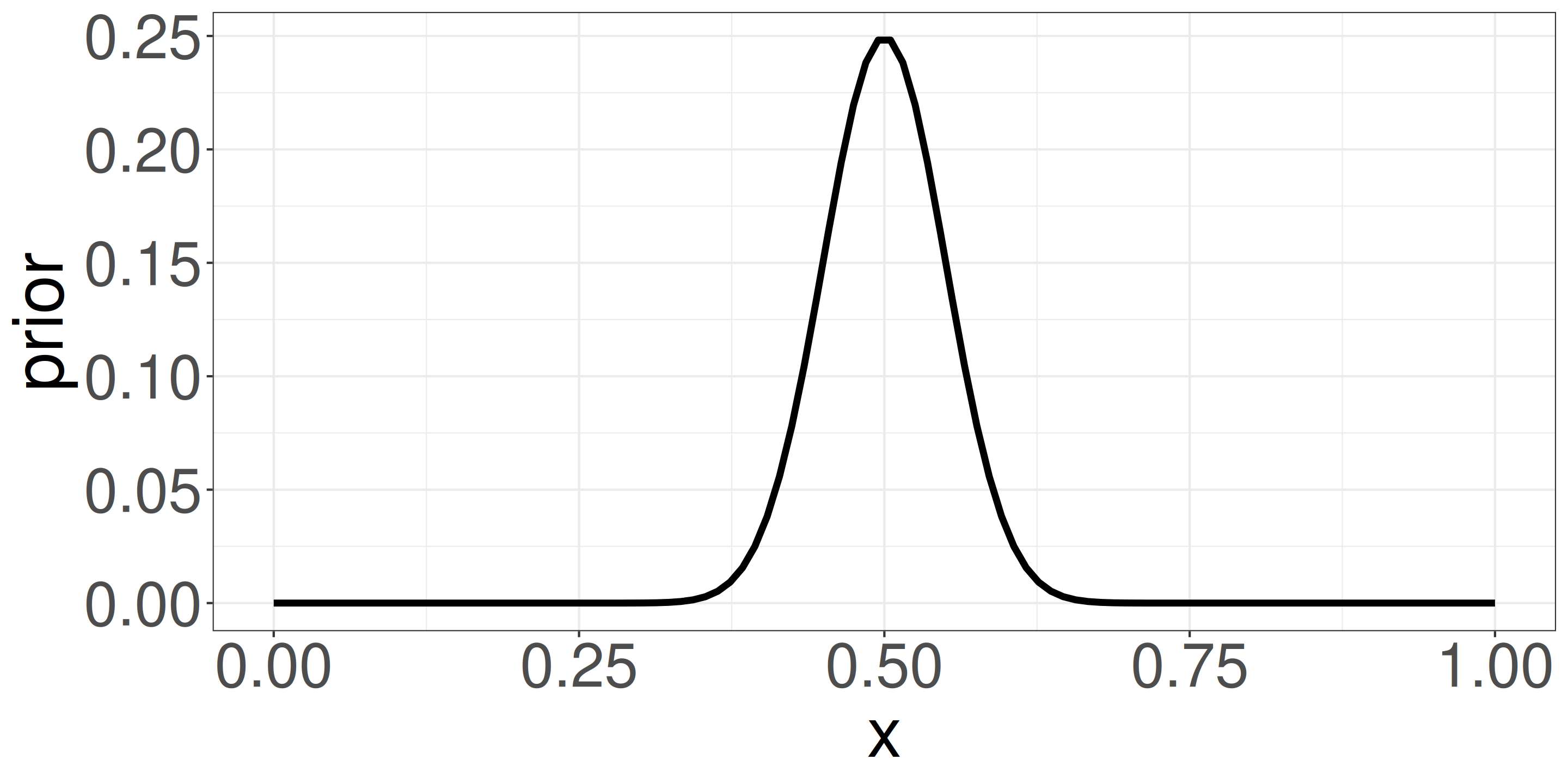
• \(\textcolor{#7570b3}{\mathrm{Prior} \propto p^{50} (1-p)^{50}}\)

  • Beta distribution with mean 0.5 and small variance (strong prior example).

Bayesian Update with Prior (Coin Toss)

Posterior \(\propto\) Likelihood \(\times\) Prior

Parameter p that maximizes the posterior of coin A. \(\textcolor{#d95f02}{Post_A}\propto\textcolor{#1b9e77}{p^2 (1-p)^1} \times\textcolor{#7570b3}{p^{50} (1-p)^{50}}\) \(p = 52/103 \approx 0.505\)

• \(Post_A\): With only 3 coin tosses, the likelihood is weak, so the posterior stays close to the prior.

Parameter p that maximizes the posterior of coin B. \(\textcolor{#d95f02}{Post_B} \propto \textcolor{#1b9e77}{p^{60} (1-p)^{40}} \times \times\textcolor{#7570b3}{p^{50} (1-p)^{50}}\) \(p = 110/200 = 0.55\)

• \(Post_B\): With 100 coin tosses, the likelihood dominates, so the posterior shifts more towards the data.

• The same prior can have a strong or weak influence depending on how much data we have.
• We usually have some sense of a scale about parameters, we can legally use that information.

Priors in ecology: Why scale matters

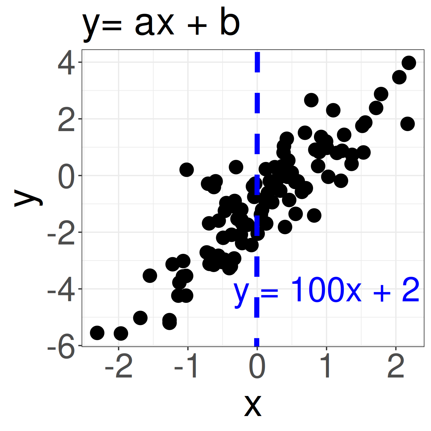
• We consider variables x = {-3, …, 3} and y = {-6, …, 4}. We don’t yet know if there is a correlation (y = ax + b).
• However, a slope like a = 100 (blue line) clearly doesn’t match the data (i.e., uninformative prior: \(a \sim \mathcal{N}(0, 10^4)\)).
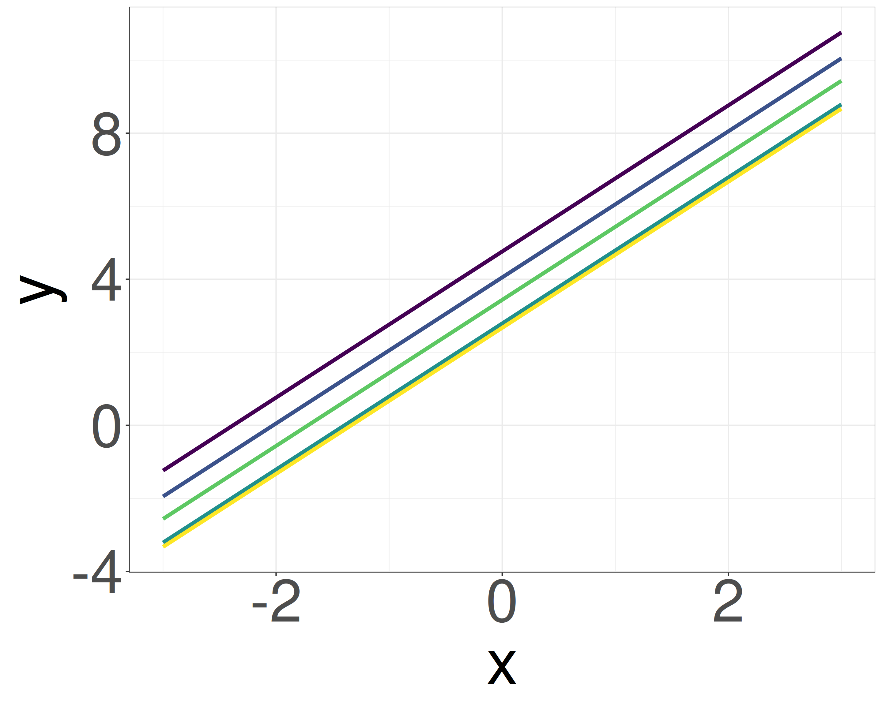
• Given the similar scales of x and y, it’s reasonable to guess that a falls within a narrow range (e.g., strongly informative prior: -5 to 5, weakly informative prior: \(a \sim \mathcal{N}(0, 2.5)\)).

Priors and ecology: multilevel structure for group-level effects

• Likelihood: \(y_i \sim \mathcal{N}(ax_i + b_j, \sigma)\)
• If the parameter \(b_j\) is similar within each group (e.g., species differences, site differences), it makes sense to model:
• Prior: \(b_j \sim \mathcal{N}(\mu_b, \tau)\)
  • \(\mu_b\): global means across all groups
  • \(\tau\): variation among groups

Priors and ecology: multilevel structure for spatial autocorrelation

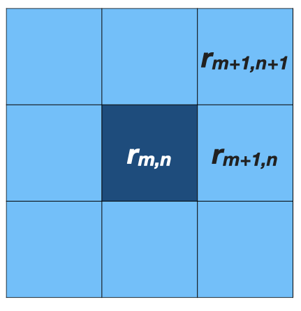
• When the data \(y_i\) is similar to the surrounding samples (e.g., temporal / spatial autocorrelation):

• Likelihood: \(y_i \sim \mathcal{N}(\mu + \tilde{r_i}, \sigma)\)
• Prior (spatial effect): \(\tilde{r_i} = r_{m, n} \sim \mathcal{N}(\phi_{m,n}, \tau)\)
• \(\phi_{m,n}\) = average of 8 neighbors around \(r_{m,n}\)

\[ \begin{align*} \phi_{m,n} = \frac{1}{8} (& r_{m-1,n-1} + r_{m-1,n} + r_{m-1,n+1} + \\ & r_{m,n-1} + r_{m,n+1} + \\ & r_{m+1,n-1} + r_{m+1,n} + r_{m+1,n+1}) \end{align*} \]

Summary: Priors

• Using weakly informative priors, we don’t have to explore the entire parameter space.

• Bayesian methods are inherently designed for hierarchical (multilevel) modeling through priors.

Multilevel model Revisit

Eight schools problem

Coaching effects in eight schools.

• s a t
• data has 8 rows with mean effects and sd of the effects
• not straightforward

Eight mother trees problem

What is the survival rate?

id	n	suv
A	41	9
B	45	18
C	32	6
D	18	5
E	33	8
F	26	8
G	46	11
H	16	8

• suv \(\sim\) B(n, p) (Binomial distribution)

• p = suv / n (Maximum likelihood estimation: MLE)

sum(dummy_simple$suv) / sum(dummy_simple$n)

  [1] 0.2840467

• If we pool all the data, the survival rate will be about 0.284

Eight mother trees problem (separate estimates)

What is the survival rate?

id	n	suv	p_like
A	41	9	0.22
B	45	18	0.40
C	32	6	0.19
D	18	5	0.28
E	33	8	0.24
F	26	8	0.31
G	46	11	0.24
H	16	8	0.50

• If we estimate each species separately, survival rates will be p_like

Eight mother trees problem (separate estimates)

What is the survival rate?

id	n	suv	p_like	p_true
A	41	9	0.22	0.34
B	45	18	0.40	0.30
C	32	6	0.19	0.34
D	18	5	0.28	0.36
E	33	8	0.24	0.25
F	26	8	0.31	0.23
G	46	11	0.24	0.25
H	16	8	0.50	0.34

• p_true ranges [0.23, 0.36]

• p_like ranges [0.19, 0.5]

• The estimate shows the larger variation

• Because of the small sample size (common in ecological studies)

• These data were simulated based on p_true, but the ML estimates are slightly different
• we want to improve the estimates

Extreme case 1: Pooled estimates

• \(S_i \sim \mathcal{B}(N_i, p)\): Likelihood
• \(\mathrm{logit}(p) \sim \mathcal{N}(0, 2.5)\): Prior

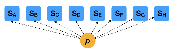
• This model assumes all mother trees share the exact same survival rate.

Extreme case 2: Separate estimates

• \(S_i \sim \mathcal{B}(N_i, p_i)\): Likelihood
• \(\mathrm{logit}(p_i) \sim \mathcal{N}(0, 2.5)\): Prior

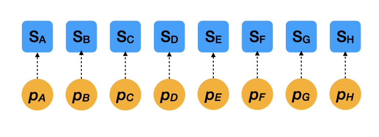
• This model assumes each mother tree has a completely independent survival rate.
• With limited data per tree, this model tends to overfit and produces noisy estimates.
• We need to find a balance between these two extremes.

• if we have infinite amount of data, we can estimate survival rates separately
• usually, we don’t have enough data (model tends to overfit)
• We need to find a balance between these two extremes

More realistic estimates: Multilevel models — partial pooling

• \(S_i \sim \mathcal{B}(N_i, p_i)\): Likelihood

• \(\mathrm{logit}(p_i) \sim \mathcal{N}(\mu, \sigma)\): Group-level model (hierarchical prior)

• \(\mu \sim \mathcal{N}(0, 2.5)\): Hyperprior

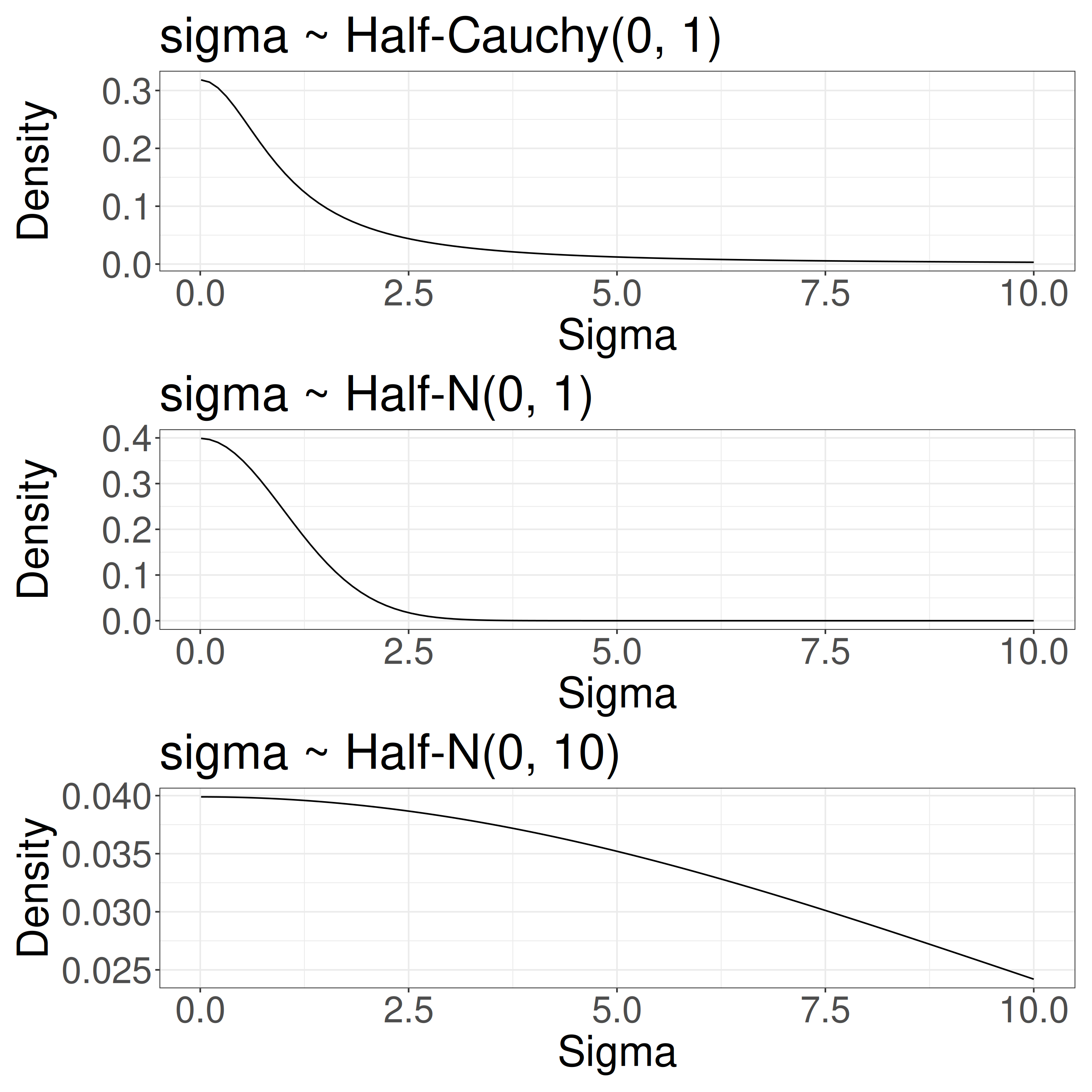
• \(\sigma \sim \text{Half-Cauchy}(0, 1)\): Hyperprior

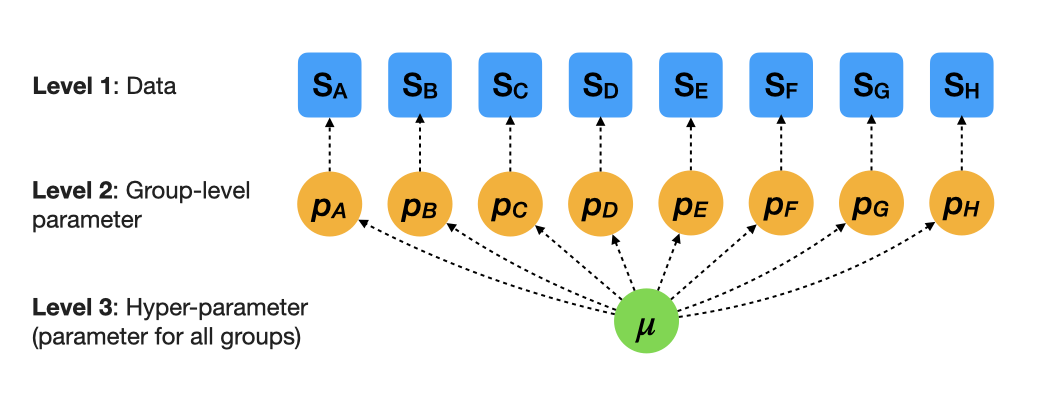
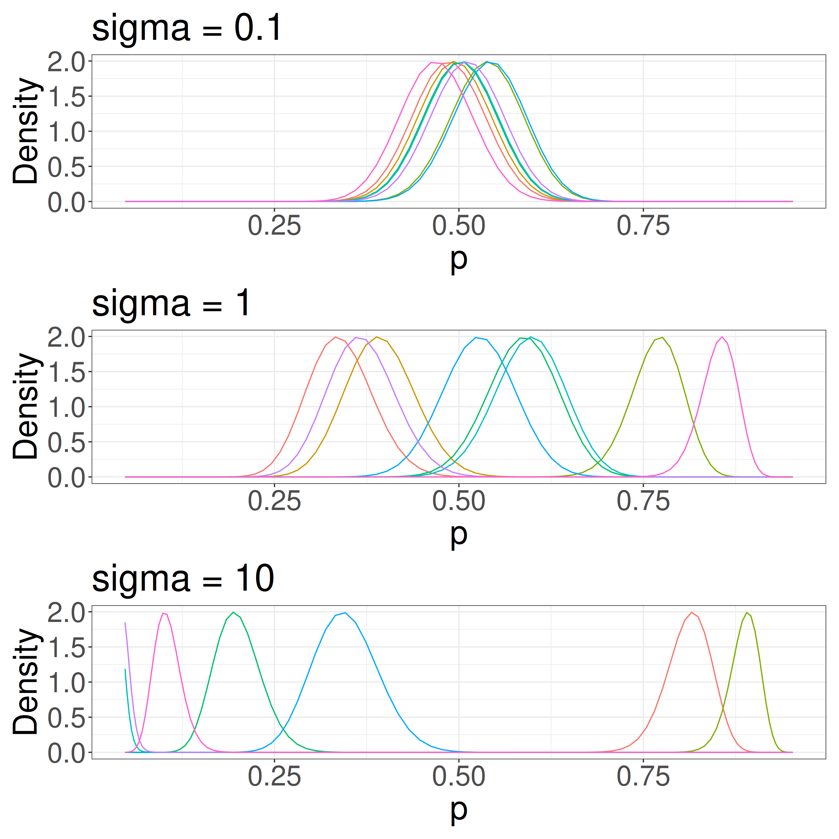
\(\sigma\) determines group-level variation

The overall survival rate is 0.5 in this figure. We have some sense of a scale for \(\sigma\).

• on the logit scale
• we have some sense of a scale for sigma
• sigma = 0.3 -> +/- 7%
• sigma = 3 -> +/- 45%
• sigma = 10 -> +/- 49.99%

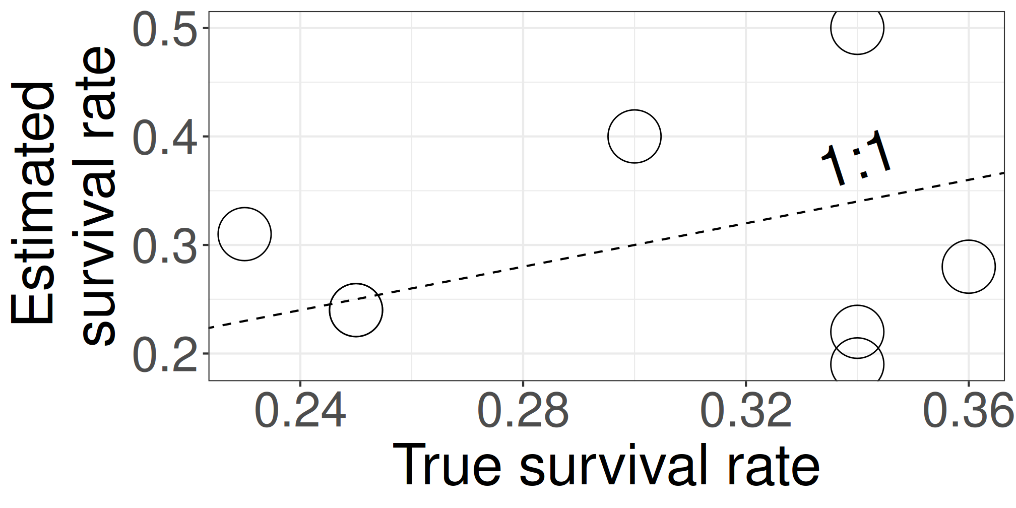
Better estimates via partial pooling (Bayesian multilevel model vs. MLE separate fits)

sp	n	suv	p_like	p_true	p_bayes
A	41	9	0.22	0.34	0.26
B	45	18	0.40	0.30	0.32
C	32	6	0.19	0.34	0.25
D	18	5	0.28	0.36	0.28
E	33	8	0.24	0.25	0.27
F	26	8	0.31	0.23	0.29
G	46	11	0.24	0.25	0.27
H	16	8	0.50	0.34	0.32

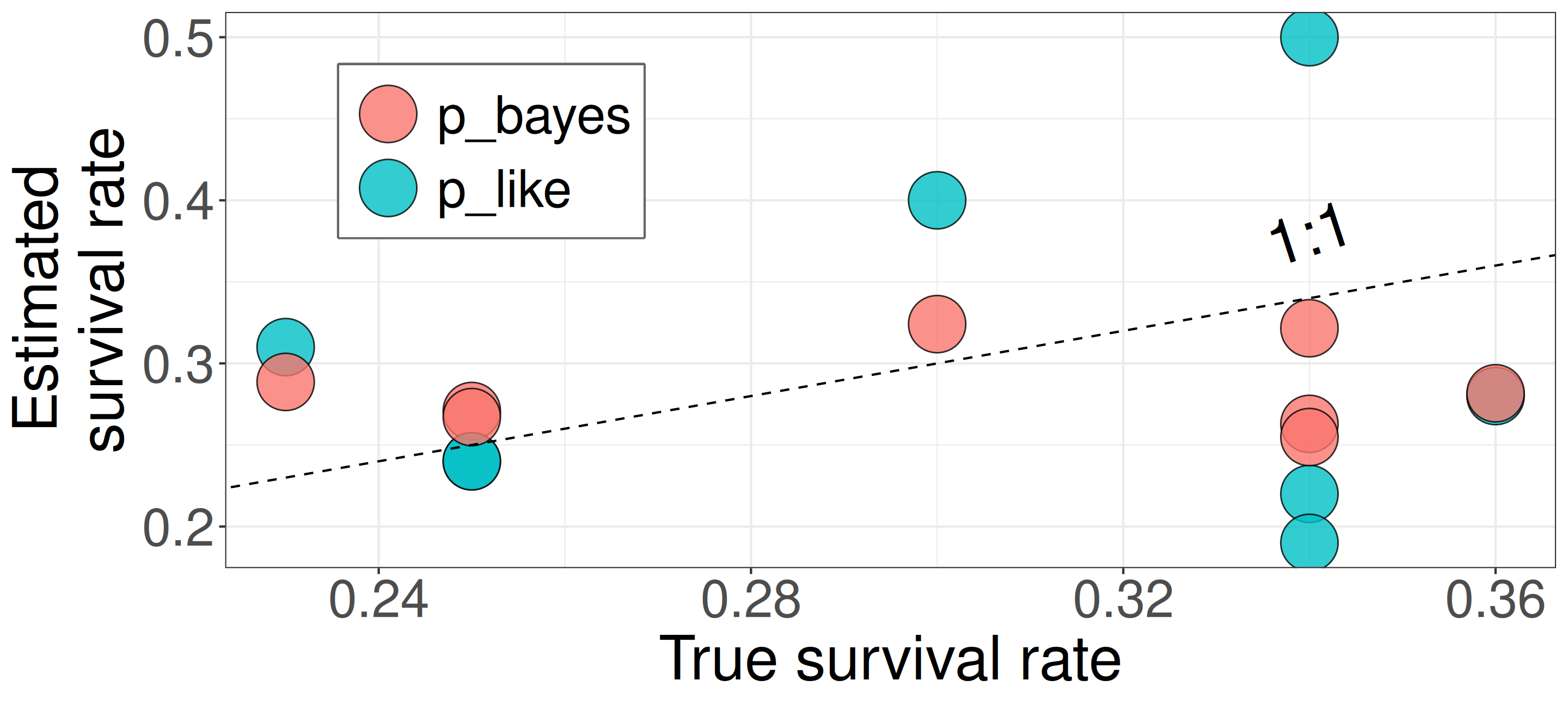
• Closed symbols (p_bayes) align more closely with the 1:1 line, indicating more accurate estimates.

• This model compensates for limited data by using prior knowledge that tree responses are somehow similar and compensates for limited data.

• less influenced by overfitting for each species

• to understand prior, we need to understand Bayes’s theorem a bit more

MLE vs. Bayesian estimation

MLE (e.g., lme4)

\(L(\mu, \sigma \mid S_i, N_i) = \prod_i \int_{-\infty}^{\infty} \mathcal{B}(S_i \mid N_i, p_i) \times \mathcal{N}(\mathrm{logit}(p_i) \mid \mu, \sigma) dp_i\)

• Analytically (or numerically) find \(\mu\) and \(\sigma\) that maximize \(L\).

• MLE often requires numerical integration, and this becomes difficult for complex models.

• No prior; estimates can be unstable or biased with small data.

MLE vs. Bayesian estimation

Bayesian estimation

\(P(\mu, \sigma \mid S_i, N_i) \propto \prod_i \mathcal{B}(S_i \mid N_i, p_i) \times \prod_i \mathcal{N}(\mathrm{logit}(p_i) \mid \mu, \sigma) \times\) \(\;\;\;\;\;\;\;\;\;\;\;\;\;\;\;\;\;\;\;\;\;\;\;\;\;\mathcal{N}(\mu \mid 0, 2.5) \times \text{Half-Cauchy}(0, 1)\)

• Use simulations (MCMC) to appoximate \(P\).

• Baesyian methods work better for complex models because they explore the full distribution instead of just finding a single best value.

• Priors help stabilize estimates, especially with limited data.

posterior distribution is proportional to the likelihood times the prior

Summary

• Why Bayesian estimation is useful.

• Why multilevel models are important.

• Bayesian workflow = Likelihood + Prior → Posterior
  • One clear pipeline for fitting, checking, and predicting.
• Priors = ecological knowledge
  • Weakly informative priors stabilize small data sets.
  • Hierarchical priors share information across species, time, sites, etc.
• Multilevel models are the default in ecology
  • Ecology is hierarchical (individual → population → community); Bayesian tools handle this naturally.

Tools for Bayesian Modeling

Tools for Bayesian Modeling

• Basic idea of MCMC
• Stan: A modern language for Bayesian modeling
• Interfaces to Stan

MCMC (Markov Chain Monte Carlo)

Goal: Approximate the posterior distribution of parameters given the data instead of calculating it directly.

For simple models, we can analytically find parameters that maximize the posterior distribution.

Coin B example again:

\(\textcolor{#d95f02}{Post_B}\propto\textcolor{#1b9e77}{p^{60} (1-p)^{40}} \times\textcolor{#7570b3}{p^{50} (1-p)^{50}}\)

\(p = 110/200 = 0.55\)

MCMC: a simplified Metropolis-Hastings (MH) algorithm

• Start with some values of p (e.g., 0.2 and 0.8).
• Caclulate the posterior of those values.
• Repeat the following steps N times:
  • Propose a new value of \(p_{\text{new}}\) (e.g., \(p \pm 0.01\))
  • Calculate the posterior at \(p_{\text{new}}\).
  • If \(\text{Post}(p_{\text{new}}) \geq \text{Post}(p_t), \text{ then } p_{t+1} = p_{\text{new}}\).
  • Else, accept \(p_{\text{new}}\) with probability \(\frac{\text{Post}(p_{\text{new}})}{\text{Post}(p_t)}\).

MCMC: Gibbs sampling

• Sampling \(\theta_1\), \(\theta_2\) jointly is hard: \(p(\theta_1, \theta_2 \mid \text{data}) \propto p(\text{data} \mid \theta_1, \theta_2) \times p(\theta_1, \theta_2)\)

• Instead, we sample \(\theta_1\) and \(\theta_2\) sequentially:

  • \(p(\theta_1 \mid \theta_2, \text{data}) \propto p(\text{data} \mid \theta_1, \theta_2) \times p(\theta_1 \mid \theta_2)\)

  • \(p(\theta_2 \mid \theta_1, \text{data}) \propto p(\text{data} \mid \theta_1, \theta_2) \times p(\theta_2 \mid \theta_1)\)

  • \(\theta_1^{(t)} \sim p(\theta_1 \mid \theta^{(t-1)}_2, \text{data})\)

  • \(\theta_2^{(t)} \sim p(\theta_2 \mid \theta^{(t)}_1, \text{data})\)

• Gibbs sampling approximates the joint posterior by sampling from these full conditionals.

• Implemented in BUGS and JAGS software.

MCMC: Hamiltonian Monte Carlo (HMC)

• \(H(\theta, r) = U(\theta) + r^2/2\) (Hamiltonian: potential energy + kinetic energy = constant)

  • \(U(\theta) = -\text{log}\; p(\theta \mid \text{data})\) ()

• Instead of sampling from \(p(\theta \mid \text{data})\), HMC samples from a joint distribution over both \(\theta\) and \(r\).

  • \(p(\theta \mid \text{data}) \propto \int \text{exp}(-H(\theta, r))dr\)

• It’s equivalent to sampling from \(p(\theta \mid \text{data}) \propto \text{exp}(-U(\theta))\).

• HMS explores very different \(\theta\) along the same trajectory (i.e. leapfrog path), which is much more efficient than random sampling.

MCMC: Hamiltonian Monte Carlo (HMC)

• Within each iteration, HMC simulates a trajectory using leapfrog steps.

  • No-U-Turn Sampler (NUTS) dynamically determines the number of leapfrog steps; we only need to set the maximum (e.g., max_treedepth in Stan).

• The Hamiltonian stays almost constant, but momentum \(r\) is resampled each iteration.

• Only the final parameter \(\theta\) of each trajectory is kept as a posterior sample.

MCMC: HMC vs. Metropolis-Hastings (MH)

MCMC Methods: Comparison

Feature	Metropolis(-Hastings)	Gibbs Sampling	Hamiltonian Monte Carlo (HMC)
How it works	Try random moves, accept/reject	Update one parameter at a time	Simulate smooth movement using gradients
Efficient in high dimensions?	❌ Often slow	✅ If math is simple	✅ Very efficient
Flexible?	✅ Yes	❌ No (conjugate priors)	✅ Yes
Typical software	JAGS, custom R	JAGS, BUGS	Stan

Stan: A modern language/software for Bayesian modeling

data {
  int<lower=0> N;
  array[N] int<lower=0, upper=1> y;
}
parameters {
  real<lower=0, upper=1> theta;
}
model {
  // uniform prior on interval 0,1
  theta ~ beta(1, 1);
  // likelihood
  y ~ bernoulli(theta);
}

• Bayesian Modeling

  • Stan uses the No-U-Turn sampler (NUTS), a variant of Hamiltonian Monte Carlo (HMC), which is efficient for complex models with many parameters.

• Flexible and Scalable

  • You can use Stan for many types of models, from simple regressions to multi-level models including time-series, spatial, SEM, and more.

• Multiplatform

  • Stan works with R, Python, Julia, and more. It also has tools for checking models and making visualizations.

Interfaces to Stan (for R users)

• Stan: The actual modeling and inference engine, written in C++.

• CmdStan: Command line interface (you write Stan code and run it via terminal).

• rstan, cmdstanr: R interface to Stan/CmdStan (you write Stan code and run it within R).

• brms, rstanarm: Higher-level R packages that depend on rstan (you write R code and run models within R, without writing Stan code).

• In this course, we will use cmdstanr and brms.

Stan Coding Session (separate HTML material)

References

• Slides & code: https://github.com/mattocci27/afec-bayes-2025

• Gelman, A. et al. Bayesian Data Analysis, Third Edition. (Chapman & Hall/CRC, 2013)

• Stan User’s Guide

• Stan Functions Reference

• AIcia Solid Project (in Japanese and Math)